In order to find the average value in Excel (no matter whether it is a numeric, text, percentage or other value), there are many functions. And each of them has its own characteristics and advantages. Indeed, in this task certain conditions may be set.
For example, the average values of a series of numbers in Excel are calculated using statistical functions. You can also manually enter your own formula. Let's consider various options.
How to find the arithmetic mean of numbers?
To find the arithmetic mean, you need to add up all the numbers in the set and divide the sum by the quantity. For example, a student’s grades in computer science: 3, 4, 3, 5, 5. What is included in the quarter: 4. We found the arithmetic mean using the formula: =(3+4+3+5+5)/5.
How to quickly do this using Excel functions? Let's take for example a series of random numbers in a string:

Or: make the active cell and simply enter the formula manually: =AVERAGE(A1:A8).
Now let's see what else the AVERAGE function can do.

Let's find the arithmetic mean of the first two and three last numbers. Formula: =AVERAGE(A1:B1,F1:H1). Result:
Condition average
The condition for finding the arithmetic mean can be a numerical criterion or a text one. We will use the function: =AVERAGEIF().
Find the arithmetic mean of numbers that are greater than or equal to 10.
Function: =AVERAGEIF(A1:A8,">=10")
 The result of using the AVERAGEIF function under the condition ">=10":
 The third argument – “Averaging range” – is omitted. First of all, it is not required. Secondly, the range analyzed by the program contains ONLY numeric values. The cells specified in the first argument will be searched according to the condition specified in the second argument.
Attention! The search criterion can be specified in the cell. And make a link to it in the formula.
Let's find the average value of the numbers using the text criterion. For example, the average sales of the product “tables”.

The function will look like this: =AVERAGEIF($A$2:$A$12,A7,$B$2:$B$12). Range – a column with product names. The search criterion is a link to a cell with the word “tables” (you can insert the word “tables” instead of link A7). Averaging range – those cells from which data will be taken to calculate the average value.
As a result of calculating the function, we obtain the following value:
Attention! For a text criterion (condition), the averaging range must be specified.
How to calculate the weighted average price in Excel?

How did we find out the weighted average price?
Formula: =SUMPRODUCT(C2:C12,B2:B12)/SUM(C2:C12).

Using the SUMPRODUCT formula, we find out the total revenue after selling the entire quantity of goods. And the SUM function sums up the quantity of goods. By dividing the total revenue from the sale of goods by the total number of units of goods, we found the weighted average price. This indicator takes into account the “weight” of each price. Its share in the total mass of values.
Standard deviation: formula in Excel
There are standard deviations for the general population and for the sample. In the first case, this is the root of the general variance. In the second - from sample variance.
To calculate this statistical indicator, a dispersion formula is compiled. The root is extracted from it. But in Excel there is a ready-made function for finding the standard deviation.

The standard deviation is tied to the scale of the source data. For figurative representation this is not enough about the variation of the analyzed range. To obtain the relative level of data scatter, the coefficient of variation is calculated:
standard deviation / arithmetic mean
The formula in Excel looks like this:
STDEV (range of values) / AVERAGE (range of values).
The coefficient of variation is calculated as a percentage. Therefore, we set the percentage format in the cell.
Average salary... Average life expectancy... Almost every day we hear these phrases used to describe many singular. But oddly enough, the “average value” is a rather insidious concept, often misleading the ordinary, inexperienced mathematical statistics, person.
What is the problem?
The average value most often means the arithmetic mean, which varies greatly under the influence of individual facts or events. And you won't get a real sense of exactly how the values you're studying are distributed.
Let's look at the classic example of the average salary.
Some abstract company has ten employees. Nine of them receive a salary of about 50,000 rubles, and one receives a salary of 1,500,000 rubles (by a strange coincidence, he is also the general director of this company).
The average value in this case will be 195,150 rubles, which you will agree is incorrect.
What methods of calculating the average are there?
The first way is to calculate the already mentioned arithmetic mean, which is the sum of all values divided by their number.

- x – arithmetic mean;
- x n – specific meaning;
- n – number of values.
- Works well with normal distribution of values in the sample;
- Easy to calculate;
- Intuitively clear.
- Does not give a real idea of the distribution of values;
- An unstable quantity that is easily subject to outliers (as in the case of the CEO).
The second way is to calculate fashion, that is, the most frequently occurring value.
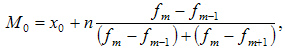
- M 0 – mode;
- x 0 – lower boundary of the interval that contains the mode;
- n – interval value;
- f m – frequency (how many times a particular value occurs in a series);
- f m-1 – frequency of the interval preceding the modal one;
- f m+1 – frequency of the interval following the modal one.
- Great for getting a sense of public opinion;
- Good for non-numeric data (season colors, best sellers, ratings);
- Easy to understand.
- Fashion may simply not exist (no repetitions);
- There can be several modes (multimodal distribution).
The third way is to calculate medians, that is, the value that divides the ordered sample into two halves and lies between them. And if there is no such value, then the arithmetic mean between the boundaries of the halves of the sample is taken as the median.

- M e – median;
- x 0 – the lower limit of the interval that contains the median;
- h – interval value;
- f i – frequency (how many times a particular value occurs in a series);
- S m-1 – sum of frequencies of intervals preceding the median;
- f m – number of values in the median interval (its frequency).
- Provides the most realistic and representative estimate;
- Resistant to emissions.
- More difficult to calculate, since the sample must be ordered before calculation.
We looked at the main methods for finding the average value, called measures of central tendency(actually there are more, but these are the most popular).
Now let's go back to our example and calculate all three options for the average using special Excel functions:
- AVERAGE(number1;[number2];…) – function for determining the arithmetic mean;
- MODE.ONE(number1;[number2];...) - mode function (in older versions of Excel MODE(number1;[number2];...) was used);
- MEDIAN(number1;[number2];...) – function for finding the median.
And here are the values we got:

In this case, mode and median characterize much better average salary in company.
But what to do when the sample contains not 10 values, as in the example, but millions? This cannot be calculated in Excel, but in the database where your data is stored, no problem.
Calculating the arithmetic mean in SQL
Everything here is quite simple, since SQL provides a special aggregate function AVG.
And to use it, just write the following query:
Calculating fashion in SQL
There is no separate function in SQL for finding a mode, but you can quickly and easily write one yourself. To do this, we need to find out which salary is most often repeated and choose the most popular one.
Let's write a request:
/* WITH TIES must be added to TOP() if the set is multimodal, that is, the set has several modes */ SELECT TOP(1) WITH TIES salary AS "Salary mode" FROM employees GROUP BY salary ORDER BY COUNT(*) DESC
Calculating the median in SQL
As with mode, SQL does not have a built-in function for calculating the median, but it does have a generic function for calculating percentiles, PERCENTILE_CONT .
It all looks like this:
/* In this case, the percentile is 0.5 and will be the median */ SELECT TOP(1) PERCENTILE_CONT(0.5) WITHIN GROUP (ORDER BY salary) OVER() AS "Median salary" FROM employees
It is better to read more about the operation of the PERCENTILE_CONT function in the Microsoft and Google BigQuery help.
Which method should I use?
From the above it follows that the median The best way to calculate the average.
But it is not always the case. If you're working with an average, then beware of a multimodal distribution:

The graph shows a bimodal distribution with two peaks. This situation may arise, for example, when voting in elections.
In this case, the arithmetic mean and median are values that are somewhere in the middle and they will not say anything about what is actually happening and it is better to immediately recognize that you are dealing with a bimodal distribution by reporting two modes.
Better yet, divide the sample into two groups and collect statistical data for each.
Conclusion:
When choosing a method for finding the average, you need to take into account the presence of outliers, as well as the normality of the distribution of values in the sample.
The final choice of the measure of central tendency always lies with the analyst.
Remember!
To find the arithmetic mean, you need to add up all the numbers and divide their sum by their number.
Find the arithmetic mean of 2, 3 and 4.
Let us denote the arithmetic mean by the letter “m”. By definition above, we find the sum of all numbers.
Divide the resulting amount by the number of numbers taken. By convention, we have three numbers.
As a result we get arithmetic mean formula:

What is the arithmetic mean used for?
In addition to the fact that it is constantly suggested to be found in lessons, finding the arithmetic mean is very useful in life.
For example, let's say you decide to sell soccer balls. But since you are new to this business, it is completely unclear at what price you should sell the balls.
Then you decide to find out at what price competitors are already selling soccer balls in your area. Let's find out prices in stores and make a table.
The prices for balls in stores turned out to be completely different. What price should we choose to sell a soccer ball?
If we choose the lowest price (290 rubles), then we will sell the goods at a loss. If you choose the highest one (360 rubles), then buyers will not buy soccer balls from us.
We need an average price. This is where it comes to the rescue average.
Let's calculate the arithmetic average of prices for soccer balls:
average price =
=
290 + 360 + 310
3
= 320
rub.960
3
Thus, we have received an average price (320 rubles), at which we can sell a soccer ball not too cheap and not too expensive.
Average driving speed
Closely related to the arithmetic mean is the concept average speed.
Observing the movement of traffic in the city, you can notice that cars either accelerate and drive at high speed, or slow down and drive at low speed.
There are many such sections along the route of vehicles. Therefore, for the convenience of calculations, the concept of average speed is used.
Remember!
The average speed of movement is the entire distance traveled divided by the entire time of movement.

Let's consider a problem at medium speed.
Problem No. 1503 from the textbook “Vilenkin 5th grade”
The car moved for 3.2 hours on a highway at a speed of 90 km/h, then 1.5 hours on a dirt road at a speed of 45 km/h, and finally 0.3 hours on a country road at a speed of 30 km/h. Find the average speed of the car along the entire route.
To calculate the average speed, you need to know the entire distance traveled by the car and the entire time the car was moving.
S 1 = V 1 t 1S 1 = 90 3.2 = 288 (km)
- highway.S 2 = V 2 t 2
S 2 = 45 · 1.5 = 67.5 (km) - dirt road.
S 3 = V 3 t 3
S 3 = 30 · 0.3 = 9 (km) - country road.
S = S 1 + S 2 + S 3
S = 288 + 67.5 + 9 = 364.5 (km) - the entire distance traveled by the car.
T = t 1 + t 2 + t 3
T = 3.2 + 1.5 + 0.3 = 5 (h) - all the time.
V av = S: t
V av = 364.5: 5 = 72.9 (km/h) — average speed car movement.
Answer: V av = 72.9 (km/h) - the average speed of the car.
In most cases, data is concentrated around some central point. Thus, to describe any set of data, it is enough to indicate the average value. Let us consider sequentially three numerical characteristics that are used to estimate the average value of the distribution: arithmetic mean, median and mode.
Average
The arithmetic mean (often called simply the mean) is the most common estimate of the mean of a distribution. It is the result of dividing the sum of all observed numerical values by their number. For a sample consisting of numbers X 1, X 2, …, Xn, sample mean (denoted by ) equals = (X 1 + X 2 + … + Xn) / n, or
where is the sample mean, n- sample size, Xi – i-th element samples.
Download the note in or format, examples in format
Consider calculating the arithmetic average of the five-year average annual returns of 15 mutual funds with very high level risk (Fig. 1).

Rice. 1. Average annual returns of 15 very high-risk mutual funds
The sample mean is calculated as follows:

This is a good return, especially compared to the 3-4% return that bank or credit union depositors received over the same time period. If we sort the returns, it is easy to see that eight funds have returns above the average, and seven - below the average. The arithmetic mean acts as the equilibrium point, so that funds with low returns balance out funds with high returns. All elements of the sample are involved in calculating the average. None of the other estimates of the mean of a distribution have this property.
When should you calculate the arithmetic mean? Since the arithmetic mean depends on all elements in the sample, the presence of extreme values significantly affects the result. In such situations, the arithmetic mean can distort the meaning of numerical data. Therefore, when describing a data set containing extreme values, it is necessary to indicate the median or the arithmetic mean and the median. For example, if we remove the RS Emerging Growth fund's returns from the sample, the sample average of the 14 funds' returns decreases by almost 1% to 5.19%.
Median
The median represents the middle value of an ordered array of numbers. If the array does not contain repeating numbers, then half of its elements will be less than, and half will be greater than, the median. If the sample contains extreme values, it is better to use the median rather than the arithmetic mean to estimate the mean. To calculate the median of a sample, it must first be ordered.
This formula is ambiguous. Its result depends on whether the number is even or odd n:
- If the sample contains an odd number of elements, the median is (n+1)/2-th element.
- If the sample contains an even number of elements, the median lies between the two middle elements of the sample and is equal to the arithmetic mean calculated over these two elements.
To calculate the median of a sample containing the returns of 15 very high-risk mutual funds, you first need to sort the raw data (Figure 2). Then the median will be opposite the number of the middle element of the sample; in our example No. 8. Excel has a special function =MEDIAN() that works with unordered arrays too.

Rice. 2. Median 15 funds
Thus, the median is 6.5. This means that the return on one half of the very high-risk funds does not exceed 6.5, and the return on the other half exceeds it. Note that the median of 6.5 is not much larger than the mean of 6.08.
If we remove the return of the RS Emerging Growth fund from the sample, then the median of the remaining 14 funds decreases to 6.2%, that is, not as significantly as the arithmetic mean (Figure 3).

Rice. 3. Median 14 funds
Fashion
The term was first coined by Pearson in 1894. Fashion is the number that occurs most often in a sample (the most fashionable). Fashion describes well, for example, typical reaction drivers at a traffic light signal to stop traffic. A classic example of the use of fashion is the choice of shoe size or wallpaper color. If a distribution has several modes, then it is said to be multimodal or multimodal (has two or more “peaks”). The multimodality of the distribution provides important information about the nature of the variable being studied. For example, in opinion polls If a variable represents a preference or attitude towards something, then multimodality can mean that there are several distinctly different opinions. Multimodality also serves as an indicator that the sample is not homogeneous and the observations may be generated by two or more “overlapping” distributions. Unlike the arithmetic mean, outliers do not affect the mode. For continuously distributed random variables, such as the average annual return of mutual funds, the mode sometimes does not exist (or makes no sense) at all. Since these indicators can take on very different values, repeating values are extremely rare.
Quartiles
Quartiles are the metrics most often used to evaluate the distribution of data when describing the properties of large numerical samples. While the median splits the ordered array in half (50% of the array's elements are less than the median and 50% are greater), quartiles split the ordered data set into four parts. The values of Q 1 , median and Q 3 are the 25th, 50th and 75th percentiles, respectively. The first quartile Q 1 is a number that divides the sample into two parts: 25% of the elements are less than, and 75% are greater than, the first quartile.
The third quartile Q 3 is a number that also divides the sample into two parts: 75% of the elements are less than, and 25% are greater than, the third quartile.
To calculate quartiles in versions of Excel before 2007, use the =QUARTILE(array,part) function. Starting from Excel 2010, two functions are used:
- =QUARTILE.ON(array,part)
- =QUARTILE.EXC(array,part)
These two functions give little different meanings(Fig. 4). For example, when calculating the quartiles of a sample containing the average annual returns of 15 very high-risk mutual funds, Q 1 = 1.8 or –0.7 for QUARTILE.IN and QUARTILE.EX, respectively. By the way, the QUARTILE function, previously used, corresponds to the modern QUARTILE.ON function. To calculate quartiles in Excel using the above formulas, the data array does not need to be ordered.

Rice. 4. Calculating quartiles in Excel
Let us emphasize again. Excel can calculate quartiles for a univariate discrete series, containing the values of a random variable. The calculation of quartiles for a frequency-based distribution is given below in the section.
Geometric mean
Unlike the arithmetic mean, the geometric mean allows you to estimate the degree of change in a variable over time. The geometric mean is the root n th degree from the work n quantities (in Excel the =SRGEOM function is used):
G= (X 1 * X 2 * … * X n) 1/n
A similar parameter is average geometric meaning rate of return is determined by the formula:
G = [(1 + R 1) * (1 + R 2) * … * (1 + R n)] 1/n – 1,
Where R i– rate of profit for i th time period.
For example, suppose the initial investment is $100,000. By the end of the first year, it falls to $50,000, and by the end of the second year it recovers to the initial level of $100,000. The rate of return of this investment over a two-year period equals 0, since the initial and final amounts of funds are equal to each other. However, the arithmetic average of the annual rates of return is = (–0.5 + 1) / 2 = 0.25 or 25%, since the rate of return in the first year R 1 = (50,000 – 100,000) / 100,000 = –0.5 , and in the second R 2 = (100,000 – 50,000) / 50,000 = 1. At the same time, the geometric mean value of the rate of profit for two years is equal to: G = [(1–0.5) * (1+1 )] 1/2 – 1 = ½ – 1 = 1 – 1 = 0. Thus, the geometric mean more accurately reflects the change (more precisely, the absence of changes) in the volume of investment over a two-year period than the arithmetic mean.
Interesting Facts. Firstly, the geometric mean will always be less than the arithmetic mean of the same numbers. Except for the case when all the numbers taken are equal to each other. Secondly, having considered the properties right triangle, one can understand why the mean is called geometric. The height of a right triangle, lowered to the hypotenuse, is the average proportional between the projections of the legs onto the hypotenuse, and each leg is the average proportional between the hypotenuse and its projection onto the hypotenuse (Fig. 5). This gives a geometric way to construct the geometric mean of two (lengths) segments: you need to construct a circle on the sum of these two segments as a diameter, then the height restored from the point of their connection to the intersection with the circle will give the desired value:

Rice. 5. Geometric nature of the geometric mean (figure from Wikipedia)
Second important property numerical data - their variation, characterizing the degree of data dispersion. Two different samples may differ in both means and variances. However, as shown in Fig. 6 and 7, two samples may have the same variations but different means, or the same means and completely different variations. The data that corresponds to polygon B in Fig. 7, change much less than the data on which polygon A was constructed.

Rice. 6. Two symmetrical bell-shaped distributions with the same spread and different mean values

Rice. 7. Two symmetrical bell-shaped distributions with the same mean values and different spreads
There are five estimates of data variation:
- scope,
- interquartile range,
- dispersion,
- standard deviation,
- the coefficient of variation.
Scope
The range is the difference between the largest and smallest elements of the sample:
Range = XMax – XMin
The range of a sample containing the average annual returns of 15 very high-risk mutual funds can be calculated using the ordered array (see Figure 4): Range = 18.5 – (–6.1) = 24.6. This means that the difference between the highest and lowest average annual returns of very high-risk funds is 24.6%.
Range measures the overall spread of data. Although sample range is a very simple estimate of the overall spread of the data, its weakness is that it does not take into account exactly how the data are distributed between the minimum and maximum elements. This effect is clearly visible in Fig. 8, which illustrates samples having the same range. Scale B demonstrates that if a sample contains at least one extreme value, the sample range is a very imprecise estimate of the spread of the data.

Rice. 8. Comparison of three samples with the same range; the triangle symbolizes the support of the scale, and its location corresponds to the sample mean
Interquartile range
The interquartile, or average, range is the difference between the third and first quartiles of the sample:
Interquartile range = Q 3 – Q 1
This value allows us to estimate the scatter of 50% of the elements and not take into account the influence of extreme elements. The interquartile range of a sample containing the average annual returns of 15 very high-risk mutual funds can be calculated using the data in Fig. 4 (for example, for the QUARTILE.EXC function): Interquartile range = 9.8 – (–0.7) = 10.5. The interval bounded by the numbers 9.8 and -0.7 is often called the middle half.
It should be noted that the values of Q 1 and Q 3 , and hence the interquartile range, do not depend on the presence of outliers, since their calculation does not take into account any value that would be less than Q 1 or greater than Q 3 . Total quantitative characteristics values such as the median, first and third quartiles, and interquartile range that are not affected by outliers are called robust measures.
Although range and interquartile range provide estimates of the overall and average spread of a sample, respectively, neither of these estimates takes into account exactly how the data are distributed. Variance and standard deviation are devoid of this drawback. These indicators allow you to assess the degree to which data fluctuates around the average value. Sample variance is an approximation of the arithmetic mean calculated from the squares of the differences between each sample element and the sample mean. For a sample X 1, X 2, ... X n, the sample variance (denoted by the symbol S 2 is given by the following formula:

IN general case sample variance is the sum of the squares of the differences between the sample elements and the sample mean, divided by a value equal to the sample size minus one:

Where - arithmetic mean, n- sample size, X i - i th selection element X. In Excel before version 2007, the =VARIN() function was used to calculate the sample variance; since version 2010, the =VARIAN() function is used.
The most practical and widely accepted estimate of the spread of data is sample standard deviation. This indicator is denoted by the symbol S and is equal to square root from sample variance:

In Excel before version 2007, the function =STDEV.() was used to calculate the standard sample deviation; since version 2010, the function =STDEV.V() is used. To calculate these functions, the data array may be unordered.
Neither the sample variance nor the sample standard deviation can be negative. The only situation in which the indicators S 2 and S can be zero is if all elements of the sample are equal to each other. In this completely improbable case, the range and interquartile range are also zero.
Numerical data is inherently volatile. Any variable can take many different meanings. For example, different mutual funds have different indicators profitability and losses. Due to the variability of numerical data, it is very important to study not only estimates of the mean, which are summary in nature, but also estimates of variance, which characterize the spread of the data.
Dispersion and standard deviation allow you to evaluate the spread of data around the average value, in other words, determine how many sample elements are less than the average and how many are greater. Dispersion has some valuable mathematical properties. However, its value is the square of the unit of measurement - square percent, square dollar, square inch, etc. Therefore, a natural measure of dispersion is the standard deviation, which is expressed in common units of income percentage, dollars, or inches.
Standard deviation allows you to estimate the amount of variation of sample elements around the average value. In almost all situations, the majority of observed values lie within the range of plus or minus one standard deviation from the mean. Consequently, knowing the arithmetic mean of the sample elements and the standard sample deviation, it is possible to determine the interval to which the bulk of the data belongs.
The standard deviation of returns for the 15 very high-risk mutual funds is 6.6 (Figure 9). This means that the profitability of the bulk of funds differs from the average value by no more than 6.6% (i.e., it fluctuates in the range from –S= 6.2 – 6.6 = –0.4 to +S= 12.8). In fact, the five-year average annual return of 53.3% (8 out of 15) of the funds lies within this range.

Rice. 9. Sample standard deviation
Note that when summing the squared differences, sample items that are further away from the mean are weighted more heavily than items that are closer to the mean. This property is the main reason why the arithmetic mean is most often used to estimate the mean of a distribution.
The coefficient of variation
Unlike previous estimates of scatter, the coefficient of variation is a relative estimate. It is always measured as a percentage and not in the units of the original data. The coefficient of variation, denoted by the symbols CV, measures the dispersion of the data around the mean. The coefficient of variation is equal to the standard deviation divided by the arithmetic mean and multiplied by 100%:

Where S- standard sample deviation, - sample average.
The coefficient of variation allows you to compare two samples whose elements are expressed in different units of measurement. For example, the manager of a mail delivery service intends to renew his fleet of trucks. When loading packages, there are two restrictions to consider: the weight (in pounds) and the volume (in cubic feet) of each package. Suppose that in a sample containing 200 bags, the mean weight is 26.0 pounds, the standard deviation of weight is 3.9 pounds, the mean bag volume is 8.8 cubic feet, and the standard deviation of volume is 2.2 cubic feet. How to compare the variation in weight and volume of packages?
Since the units of measurement for weight and volume differ from each other, the manager must compare the relative spread of these quantities. The coefficient of variation of weight is CV W = 3.9 / 26.0 * 100% = 15%, and the coefficient of variation of volume is CV V = 2.2 / 8.8 * 100% = 25%. Thus, the relative variation in the volume of packets is much greater than the relative variation in their weight.
Distribution form
The third important property of a sample is the shape of its distribution. This distribution may be symmetrical or asymmetrical. To describe the shape of a distribution, it is necessary to calculate its mean and median. If the two are the same, the variable is considered symmetrically distributed. If the mean value of a variable is greater than the median, its distribution has a positive skewness (Fig. 10). If the median is greater than the mean, the distribution of the variable is negatively skewed. Positive skewness occurs when the mean increases to unusually high values. Negative skewness occurs when the mean decreases to unusually small values. A variable is symmetrically distributed if it does not take any extreme values in either direction, so that large and small values of the variable cancel each other out.

Rice. 10. Three types of distributions
Data shown on scale A are negatively skewed. This figure shows a long tail and a leftward skew caused by the presence of unusually small values. These extremely small values shift the average value to the left, making it less than the median. The data shown on scale B is distributed symmetrically. The left and right halves of the distribution are their own mirror reflections. Large and small values balance each other, and the mean and median are equal. The data shown on scale B is positively skewed. This figure shows a long tail and a skew to the right caused by the presence of unusually high values. These too large values shift the mean to the right, making it larger than the median.
In Excel, descriptive statistics can be obtained using an add-in Analysis package. Go through the menu Data → Data analysis, in the window that opens, select the line Descriptive Statistics and click Ok. In the window Descriptive Statistics be sure to indicate Input interval(Fig. 11). If you want to see descriptive statistics on the same sheet as the original data, select the radio button Output interval and specify the cell where the upper left corner of the displayed statistics should be placed (in our example, $C$1). If you want to output data to a new sheet or to new book, just select the appropriate switch. Check the box next to Summary statistics. If desired, you can also choose Difficulty level,kth smallest andkth largest.
If on deposit Data in area Analysis you don't see the icon Data analysis, you need to install the add-on first Analysis package(see, for example,).

Rice. 11. Descriptive statistics of five-year average annual returns of funds with very high levels of risk, calculated using the add-in Data analysis Excel programs
Excel calculates a number of statistics discussed above: mean, median, mode, standard deviation, variance, range ( interval), minimum, maximum and sample size ( check). Excel also calculates some statistics that are new to us: standard error, kurtosis, and skewness. Standard error equal to the standard deviation divided by the square root of the sample size. Asymmetry characterizes the deviation from the symmetry of the distribution and is a function that depends on the cube of the differences between the sample elements and the average value. Kurtosis is a measure of the relative concentration of data around the mean compared to the tails of the distribution and depends on the differences between the sample elements and the mean raised to the fourth power.
Calculating descriptive statistics for a population
The mean, spread, and shape of the distribution discussed above are characteristics determined from the sample. However, if the data set contains numerical measurements of the entire population, its parameters can be calculated. Such parameters include the expected value, dispersion and standard deviation of the population.
Expected value equal to the sum of all values in the population divided by the size of the population:

Where µ - expected value, Xi- i th observation of the variable X, N- volume of the general population. In Excel, to calculate the mathematical expectation, the same function is used as for the arithmetic average: =AVERAGE().
Population variance equal to the sum of the squares of the differences between the elements of the general population and the mat. expectation divided by the size of the population:

Where σ 2– dispersion of the general population. In Excel prior to version 2007, the function =VARP() is used to calculate the variance of a population, starting with version 2010 =VARP().
Population standard deviation equal to the square root of the population variance:

In Excel prior to version 2007, the =STDEV() function is used to calculate the standard deviation of a population, starting with version 2010 =STDEV.Y(). Note that the formulas for the population variance and standard deviation are different from the formulas for calculating the sample variance and standard deviation. When calculating sample statistics S 2 And S the denominator of the fraction is n – 1, and when calculating parameters σ 2 And σ - volume of the general population N.
Rule of thumb
In most situations, a large proportion of observations are concentrated around the median, forming a cluster. In data sets with positive skewness, this cluster is located to the left (i.e., below) the mathematical expectation, and in sets with negative skewness, this cluster is located to the right (i.e., above) the mathematical expectation. For symmetric data, the mean and median are the same, and observations cluster around the mean, forming a bell-shaped distribution. If the distribution is not clearly skewed and the data is concentrated around a center of gravity, a rule of thumb that can be used to estimate variability is that if the data has a bell-shaped distribution, then approximately 68% of the observations are within one standard deviation of the expected value. approximately 95% of observations are no more than two standard deviations away from the mathematical expectation and 99.7% of observations are no more than three standard deviations away from the mathematical expectation.
Thus, the standard deviation, which is an estimate of the average variation around the expected value, helps to understand how observations are distributed and to identify outliers. The rule of thumb is that for bell-shaped distributions, only one value in twenty differs from the mathematical expectation by more than two standard deviations. Therefore, values outside the interval µ ± 2σ, can be considered outliers. In addition, only three out of 1000 observations differ from the mathematical expectation by more than three standard deviations. Thus, values outside the interval µ ± 3σ are almost always outliers. For distributions that are highly skewed or not bell-shaped, the Bienamay-Chebyshev rule of thumb can be applied.
More than a hundred years ago, mathematicians Bienamay and Chebyshev independently discovered useful property standard deviation. They found that for any data set, regardless of the shape of the distribution, the percentage of observations that lie within a distance of k standard deviations from mathematical expectation, not less (1 – 1/ k 2)*100%.
For example, if k= 2, the Bienname-Chebyshev rule states that at least (1 – (1/2) 2) x 100% = 75% of observations must lie in the interval µ ± 2σ. This rule is true for any k, exceeding one. The Bienamay-Chebyshev rule is very general and valid for distributions of any type. It specifies the minimum number of observations, the distance from which to the mathematical expectation does not exceed a specified value. However, if the distribution is bell-shaped, the rule of thumb more accurately estimates the concentration of data around the expected value.
Calculating Descriptive Statistics for a Frequency-Based Distribution
If the original data are not available, the frequency distribution becomes the only source of information. In such situations, it is possible to calculate approximate values of quantitative indicators of the distribution, such as the arithmetic mean, standard deviation, and quartiles.
If sample data is represented as a frequency distribution, an approximation of the arithmetic mean can be calculated by assuming that all values within each class are concentrated at the class midpoint:

Where - sample average, n- number of observations, or sample size, With- number of classes in the frequency distribution, m j- midpoint j th class, fj- frequency corresponding j-th class.
To calculate the standard deviation from a frequency distribution, it is also assumed that all values within each class are concentrated at the class midpoint.

To understand how quartiles of a series are determined based on frequencies, consider the calculation of the lower quartile based on data for 2013 on the distribution of the Russian population by average per capita monetary income (Fig. 12).

Rice. 12. Share of the Russian population with average per capita cash income per month, rubles
To calculate the first quartile of the interval variation series you can use the formula:

where Q1 is the value of the first quartile, xQ1 is the lower limit of the interval containing the first quartile (the interval is determined by the accumulated frequency that first exceeds 25%); i – interval value; Σf – sum of frequencies of the entire sample; probably always equal to 100%; SQ1–1 – accumulated frequency of the interval preceding the interval containing the lower quartile; fQ1 – frequency of the interval containing the lower quartile. The formula for the third quartile differs in that in all places you need to use Q3 instead of Q1, and substitute ¾ instead of ¼.
In our example (Fig. 12), the lower quartile is in the range 7000.1 – 10,000, the accumulated frequency of which is 26.4%. The lower limit of this interval is 7000 rubles, the value of the interval is 3000 rubles, the accumulated frequency of the interval preceding the interval containing the lower quartile is 13.4%, the frequency of the interval containing the lower quartile is 13.0%. Thus: Q1 = 7000 + 3000 * (¼ * 100 – 13.4) / 13 = 9677 rub.
Pitfalls Associated with Descriptive Statistics
In this post, we looked at how to describe a data set using various statistics that evaluate its mean, spread, and distribution. The next step is data analysis and interpretation. Until now, we have studied the objective properties of data, and now we move on to their subjective interpretation. The researcher faces two mistakes: an incorrectly chosen subject of analysis and an incorrect interpretation of the results.
The analysis of the returns of 15 very high-risk mutual funds is quite unbiased. He led to completely objective conclusions: all mutual funds have different returns, the spread of fund returns ranges from -6.1 to 18.5, and the average return is 6.08. Objectivity of data analysis is ensured the right choice total quantitative indicators of distribution. Several methods for estimating the mean and scatter of data were considered, and their advantages and disadvantages were indicated. How do you choose the right statistics to provide an objective and impartial analysis? If the data distribution is slightly skewed, should you choose the median rather than the mean? Which indicator more accurately characterizes the spread of data: standard deviation or range? Should we point out that the distribution is positively skewed?
On the other hand, data interpretation is a subjective process. Different people come to different conclusions when interpreting the same results. Everyone has their own point of view. Someone considers the total average annual returns of 15 funds with a very high level of risk to be good and is quite satisfied with the income received. Others may feel that these funds have too low returns. Thus, subjectivity should be compensated by honesty, neutrality and clarity of conclusions.
Ethical issues
Data analysis is inextricably linked to ethical issues. You should be critical of information disseminated by newspapers, radio, television and the Internet. Over time, you will learn to be skeptical not only of the results, but also of the goals, subject matter and objectivity of the research. The famous British politician Benjamin Disraeli said it best: “There are three kinds of lies: lies, damned lies and statistics.”
As noted in the note, ethical issues arise when choosing the results that should be presented in the report. Both positive and negative results should be published. In addition, when making a report or written report, the results must be presented honestly, neutrally and objectively. There is a distinction to be made between unsuccessful and dishonest presentations. To do this, it is necessary to determine what the speaker's intentions were. Sometimes the speaker omits important information out of ignorance, and sometimes it is deliberate (for example, if he uses the arithmetic mean to estimate the average of clearly skewed data to obtain the desired result). It is also dishonest to suppress results that do not correspond to the researcher's point of view.
Materials from the book Levin et al. Statistics for Managers are used. – M.: Williams, 2004. – p. 178–209
The QUARTILE function has been retained for compatibility with earlier versions of Excel.
In mathematics, the arithmetic mean of numbers (or simply the average) is the sum of all the numbers in a given set divided by the number of numbers. This is the most generalized and widespread concept of average value. As you already understood, to find the average, you need to sum up all the numbers given to you, and divide the resulting result by the number of terms.
What is the arithmetic mean?
Let's look at an example.
Example 1. Given numbers: 6, 7, 11. You need to find their average value.
Solution.
First, let's find the sum of all these numbers.
Now divide the resulting sum by the number of terms. Since we have three terms, we will therefore divide by three.
Therefore, the average of the numbers 6, 7 and 11 is 8. Why 8? Yes, because the sum of 6, 7 and 11 will be the same as three eights. This can be clearly seen in the illustration.
The average is a bit like “evening out” a series of numbers. As you can see, the piles of pencils have become the same level.
Let's look at another example to consolidate the knowledge gained.
Example 2. Given numbers: 3, 7, 5, 13, 20, 23, 39, 23, 40, 23, 14, 12, 56, 23, 29. You need to find their arithmetic mean.
Solution.
Find the amount.
3 + 7 + 5 + 13 + 20 + 23 + 39 + 23 + 40 + 23 + 14 + 12 + 56 + 23 + 29 = 330
Divide by the number of terms (in this case - 15).
Therefore, the average value of this series of numbers is 22.
Now let's consider negative numbers. Let's remember how to summarize them. For example, you have two numbers 1 and -4. Let's find their sum.
1 + (-4) = 1 – 4 = -3
Knowing this, let's look at another example.
Example 3. Find the average value of a series of numbers: 3, -7, 5, 13, -2.
Solution.
Find the sum of numbers.
3 + (-7) + 5 + 13 + (-2) = 12
Since there are 5 terms, divide the resulting sum by 5.
Therefore, the arithmetic mean of the numbers 3, -7, 5, 13, -2 is 2.4.
 In our time of technological progress, it is much more convenient to use to find the average value computer programs. Microsoft Office Excel is one of them. Finding the average in Excel is quick and easy. Moreover, this program is included in the Microsoft Office software package. Let's look at a brief instruction on how to find the arithmetic mean using this program.
In order to calculate the average value of a series of numbers, you must use the AVERAGE function. The syntax for this function is:
= Average(argument1, argument2, ... argument255)
where argument1, argument2, ... argument255 are either numbers or cell references (by cells we mean ranges and arrays).
To make it more clear, let’s try out the knowledge we have gained.


- Enter the numbers 11, 12, 13, 14, 15, 16 in cells C1 – C6.
- Select cell C7 by clicking on it. In this cell we will display the average value.
- Click on the Formulas tab.
- Select More Functions > Statistical to open the drop-down list.
- Select AVERAGE. After this, a dialog box should open.
- Select and drag cells C1 through C6 there to set the range in the dialog box.
- Confirm your actions with the "OK" button.
- If you did everything correctly, you should have the answer in cell C7 - 13.7. When you click on cell C7, the function (=Average(C1:C6)) will appear in the formula bar.
This feature is very useful for accounting, invoices, or when you just need to find the average of a very long series of numbers. Therefore, it is often used in offices and large companies. This allows you to keep your records in order and makes it possible to quickly calculate something (for example, average monthly income). You can also use Excel to find the average value of a function.
Average
This term has other meanings, see average meaning.Average(in mathematics and statistics) sets of numbers - the sum of all numbers divided by their number. It is one of the most common measures of central tendency.
It was proposed (along with the geometric mean and harmonic mean) by the Pythagoreans.
Special cases of the arithmetic mean are the mean (general population) and the sample mean (sample).
Introduction
Let us denote the set of data X = (x 1 , x 2 , …, x n), then the sample mean is usually indicated by a horizontal bar over the variable (x ¯ (\displaystyle (\bar (x))), pronounced " x with a line").
The Greek letter μ is used to denote the arithmetic mean of the entire population. For a random variable for which the mean value is determined, μ is probabilistic average or the mathematical expectation of a random variable. If the set X is a collection of random numbers with a probabilistic mean μ, then for any sample x i from this set μ = E( x i) is the mathematical expectation of this sample.
In practice, the difference between μ and x ¯ (\displaystyle (\bar (x))) is that μ is a typical variable because you can see a sample rather than the entire population. Therefore, if the sample is represented randomly (in terms of probability theory), then x ¯ (\displaystyle (\bar (x))) (but not μ) can be treated as a random variable having a probability distribution on the sample (the probability distribution of the mean).
Both of these quantities are calculated in the same way:
X ¯ = 1 n ∑ i = 1 n x i = 1 n (x 1 + ⋯ + x n) . (\displaystyle (\bar (x))=(\frac (1)(n))\sum _(i=1)^(n)x_(i)=(\frac (1)(n))(x_ (1)+\cdots +x_(n)).)
If X is a random variable, then the mathematical expectation X can be considered as the arithmetic mean of values in repeated measurements of a quantity X. This is a manifestation of the law large numbers. Therefore, the sample mean is used to estimate the unknown expected value.
It has been proven in elementary algebra that the mean n+ 1 numbers above average n numbers if and only if the new number is greater than the old average, less if and only if the new number is less than the average, and does not change if and only if the new number is equal to the average. The more n, the smaller the difference between the new and old averages.
Note that there are several other "averages" available, including the power mean, the Kolmogorov mean, the harmonic mean, the arithmetic-geometric mean, and various weighted averages (e.g., weighted arithmetic mean, weighted geometric mean, weighted harmonic mean).
Examples
- For three numbers, you need to add them and divide by 3:
- For four numbers, you need to add them and divide by 4:
Or simpler 5+5=10, 10:2. Because we were adding 2 numbers, which means how many numbers we add, we divide by that many.
Continuous random variable
For a continuously distributed quantity f (x) (\displaystyle f(x)), the arithmetic mean on the interval [ a ; b ] (\displaystyle ) is determined through a definite integral:
F (x) ¯ [ a ; b ] = 1 b − a ∫ a b f (x) d x (\displaystyle (\overline (f(x)))_()=(\frac (1)(b-a))\int _(a)^(b) f(x)dx)
Some problems of using the average
Lack of robustness
Main article: Robustness in statisticsAlthough arithmetic means are often used as averages or central tendencies, this concept is not a robust statistic, meaning that the arithmetic mean is heavily influenced by "large deviations." It is noteworthy that for distributions with a large coefficient of skewness, the arithmetic mean may not correspond to the concept of “mean”, and the values of the mean from robust statistics (for example, the median) may better describe the central tendency.
A classic example is calculating average income. The arithmetic mean can be misinterpreted as a median, which may lead to the conclusion that there are more people with higher incomes than there actually are. “Average” income is interpreted to mean that most people have incomes around this number. This “average” (in the sense of the arithmetic mean) income is higher than the incomes of most people, since a high income with a large deviation from the average makes the arithmetic mean highly skewed (in contrast, the average income at the median “resists” such skew). However, this "average" income says nothing about the number of people near the median income (and says nothing about the number of people near the modal income). However, if you take the concepts of “average” and “most people” lightly, you can draw the incorrect conclusion that most people have incomes higher than they actually are. For example, a report of the "average" net income in Medina, Washington, calculated as the arithmetic average of all annual net incomes of the residents, will surprisingly yield big number because of Bill Gates. Consider the sample (1, 2, 2, 2, 3, 9). The arithmetic mean is 3.17, but five out of six values are below this mean.
Compound interest
Main article: Return on InvestmentIf the numbers multiply, but not fold, you need to use the geometric mean, not the arithmetic mean. Most often this incident occurs when calculating the return on investment in finance.
For example, if a stock fell 10% in the first year and rose 30% in the second, then it is incorrect to calculate the “average” increase over those two years as the arithmetic mean (−10% + 30%) / 2 = 10%; the correct average in this case is given by the compound annual growth rate, which gives an annual growth rate of only about 8.16653826392% ≈ 8.2%.
The reason for this is that percentages have a new starting point each time: 30% is 30% from a number less than the price at the beginning of the first year: if a stock started out at $30 and fell 10%, it is worth $27 at the start of the second year. If the stock rose 30%, it would be worth $35.1 at the end of the second year. The arithmetic average of this growth is 10%, but since the stock has only risen by $5.1 over 2 years, the average growth of 8.2% gives a final result of $35.1:
[$30 (1 - 0.1) (1 + 0.3) = $30 (1 + 0.082) (1 + 0.082) = $35.1]. If we use the arithmetic average of 10% in the same way, we will not get the actual value: [$30 (1 + 0.1) (1 + 0.1) = $36.3].
Compound interest at the end of 2 years: 90% * 130% = 117%, that is, the total increase is 17%, and the average annual compound interest is 117% ≈ 108.2% (\displaystyle (\sqrt (117\%))\approx 108.2\%) , that is, an average annual increase of 8.2%.
Directions
Main article: Destination statisticsWhen calculating the arithmetic mean of some variable that changes cyclically (such as phase or angle), special care must be taken. For example, the average of 1° and 359° would be 1 ∘ + 359 ∘ 2 = (\displaystyle (\frac (1^(\circ )+359^(\circ ))(2))=) 180°. This number is incorrect for two reasons.
- Firstly, angular measures are defined only for the range from 0° to 360° (or from 0 to 2π when measured in radians). So the same pair of numbers could be written as (1° and −1°) or as (1° and 719°). The average values of each pair will be different: 1 ∘ + (− 1 ∘) 2 = 0 ∘ (\displaystyle (\frac (1^(\circ )+(-1^(\circ )))(2))=0 ^(\circ )) , 1 ∘ + 719 ∘ 2 = 360 ∘ (\displaystyle (\frac (1^(\circ )+719^(\circ ))(2))=360^(\circ )) .
- Second, in this case, a value of 0° (equivalent to 360°) will be a geometrically better average value, since the numbers deviate less from 0° than from any other value (the value 0° has the smallest variance). Compare:
- the number 1° deviates from 0° by only 1°;
- the number 1° deviates from the calculated average of 180° by 179°.
The average value for a cyclic variable calculated using the above formula will be artificially shifted relative to the real average towards the middle of the numerical range. Because of this, the average is calculated in a different way, namely, the number with the smallest variance (the center point) is selected as the average value. Also, instead of subtraction, the modular distance (that is, the circumferential distance) is used. For example, the modular distance between 1° and 359° is 2°, not 358° (on the circle between 359° and 360°==0° - one degree, between 0° and 1° - also 1°, in total - 2 °).
Weighted average - what is it and how to calculate it?
In the process of studying mathematics, schoolchildren become familiar with the concept of arithmetic mean. Later in statistics and some other sciences, students are faced with the calculation of other average values. What can they be and how do they differ from each other?
Averages: meaning and differences
Accurate indicators do not always provide an understanding of the situation. In order to assess a particular situation, it is sometimes necessary to analyze great amount numbers And then averages come to the rescue. They allow us to assess the situation as a whole.

 Since school days, many adults remember the existence of the arithmetic mean. It is very simple to calculate - the sum of a sequence of n terms is divided by n. That is, if you need to calculate the arithmetic mean in the sequence of values 27, 22, 34 and 37, then you need to solve the expression (27+22+34+37)/4, since 4 values are used in the calculations. In this case, the required value will be 30.
Often within school course Geometric mean is also studied. The calculation of this value is based on extracting the nth root of the product of n terms. If we take the same numbers: 27, 22, 34 and 37, then the result of the calculations will be equal to 29.4.
Harmonic mean in secondary school is not usually the subject of study. However, it is used quite often. This value is the inverse of the arithmetic mean and is calculated as the quotient of n - the number of values and the sum 1/a 1 +1/a 2 +...+1/a n. If we again take the same series of numbers for calculation, then the harmonic will be 29.6.


Weighted average: features
However, all of the above values may not be used everywhere. For example, in statistics, when calculating certain averages, the “weight” of each number used in the calculations plays an important role. The results are more indicative and correct, since they take into account more information. This group of quantities is common name"weighted average". They are not taught in school, so it is worth looking at them in more detail.
First of all, it is worth telling what is meant by the “weight” of a particular value. The easiest way to explain this is specific example. Twice a day in the hospital the body temperature of each patient is measured. Out of 100 patients in different departments of the hospital, 44 will have a normal temperature - 36.6 degrees. Another 30 will have an increased value - 37.2, 14 - 38, 7 - 38.5, 3 - 39, and the remaining two - 40. And if we take the arithmetic average, then this value in general for the hospital will be more than 38 degrees! But almost half of the patients have a completely normal temperature. And here it would be more correct to use a weighted average, and the “weight” of each value would be the number of people. In this case, the calculation result will be 37.25 degrees. The difference is obvious.
In the case of weighted average calculations, the “weight” can be taken as the number of shipments, the number of people working on a given day, in general, anything that can be measured and affect the final result.


Varieties
The weighted average is related to the arithmetic mean discussed at the beginning of the article. However, the first value, as already mentioned, also takes into account the weight of each number used in the calculations. In addition, there are also weighted geometric and harmonic values.
There is another interesting variation used in number series. It's about about a weighted moving average. It is on this basis that trends are calculated. In addition to the values themselves and their weight, periodicity is also used there. And when calculating the average value at some point in time, values for previous time periods are also taken into account.
Calculating all these values is not that difficult, but in practice only the ordinary weighted average is usually used.
Calculation methods
In the age of widespread computerization, there is no need to calculate the weighted average manually. However, it would be useful to know the calculation formula so that you can check and, if necessary, adjust the results obtained.
The easiest way is to consider the calculation using a specific example.
It is necessary to find out what the average wage is at this enterprise, taking into account the number of workers receiving one or another salary.
So, the weighted average is calculated using the following formula:
x = (a 1 *w 1 +a 2 *w 2 +...+a n *w n)/(w 1 +w 2 +...+w n)
For example, the calculation would be like this:
x = (32*20+33*35+34*14+40*6)/(20+35+14+6) = (640+1155+476+240)/75 = 33.48
Obviously, there is no particular difficulty in manually calculating the weighted average. The formula for calculating this value in one of the most popular applications with formulas - Excel - looks like the SUMPRODUCT (series of numbers; series of weights) / SUM (series of weights) function.
How to find the average in excel?
how to find the arithmetic mean in excel?
Vladimir09854
As easy as pie. To find the average in excel, you only need 3 cells. In the first we will write one number, in the second - another. And in the third cell we will enter a formula that will give us the average value between these two numbers from the first and second cells. If cell No. 1 is called A1, cell No. 2 is called B1, then in the cell with the formula you need to write this:
This formula calculates the arithmetic mean of two numbers.
To make our calculations more beautiful, we can highlight the cells with lines, in the form of a plate.
In Excel itself there is also a function for determining the average value, but I use the old-fashioned method and enter the formula I need. Thus, I am sure that Excel will calculate exactly as I need, and will not come up with some kind of rounding of its own.
M3sergey
This is very simple if the data is already entered into the cells. If you are interested in just a number, just select the desired range/ranges, and the value of the sum of these numbers, their arithmetic mean and their number will appear at the bottom right in the status bar.
You can select an empty cell, click on the triangle (drop-down list) “AutoSum” and select “Average” there, after which you will agree with the proposed range for calculation, or select your own.
Finally, you can use formulas directly by clicking "Insert Function" next to the formula bar and cell address. The AVERAGE function is located in the “Statistical” category, and takes as arguments both numbers and cell references, etc. There you can also select more complex options, for example, AVERAGEIF - calculating the average according to the condition.
Find average value in excel is a fairly simple task. Here you need to understand whether you want to use this average value in some formulas or not.
If you only need to get the value, then just select the required range of numbers, after which Excel will automatically calculate the average value - it will be displayed in the status bar, the heading "Average".
In the case when you want to use the result in formulas, you can do this:
1) Sum the cells using the SUM function and divide it all by the number of numbers.


2) A more correct option is to use a special function called AVERAGE. The arguments to this function can be numbers specified sequentially or a range of numbers.


Vladimir Tikhonov
Circle the values that will participate in the calculation, click the “Formulas” tab, there you will see on the left there is “AutoSum” and next to it a triangle pointing down. Click on this triangle and select "Medium". Voila, done) at the bottom of the column you will see the average value :)
Ekaterina Mutalapova
Let's start from the beginning and in order. What does average mean?
The mean is a value that is the arithmetic mean, i.e. is calculated by adding a set of numbers and then dividing the entire sum of numbers by their number. For example, for the numbers 2, 3, 6, 7, 2 there will be 4 (the sum of the numbers 20 is divided by their number 5)
In an Excel spreadsheet, for me personally, the easiest way was to use the formula = AVERAGE. To calculate the average value, you need to enter data into the table, write the function =AVERAGE() under the data column, and indicate the range of numbers in the cells in brackets, highlighting the column with the data. After that, press ENTER, or simply left-click on any cell. The result appears in the cell below the column. It looks incomprehensibly described, but in fact it’s a matter of minutes.
Adventurer 2000
Excel is a varied program, so there are several options that will allow you to find averages:
First option. You simply sum all the cells and divide by their number;
Second option. Use a special command, write the formula “= AVERAGE (and here indicate the range of cells)” in the required cell;
Third option. If you select the required range, please note that on the page below, the average value in these cells is also displayed.
Thus, there are a lot of ways to find the average, you just need to choose the best one for you and use it constantly.
In Excel, you can use the AVERAGE function to calculate the simple arithmetic average. To do this, you need to enter a number of values. Press equals and select Statistical in the Category, among which select the AVERAGE function


Also, using statistical formulas, you can calculate the weighted arithmetic mean, which is considered more accurate. To calculate it, we need indicator values and frequency.
How to find the average in Excel?
This is the situation. There is the following table:
The columns shaded in red contain the numerical values of grades in subjects. In the column " Average score"It is necessary to calculate their average value.
The problem is this: there are 60-70 items in total and some of them are on another sheet.
I looked in another document and the average has already been calculated, and in the cell there is a formula like
="sheet name"!|E12
but this was done by some programmer who was fired.
Please tell me who understands this.
Hector
In the functions line, you insert “AVERAGE” from the proposed functions and select where they need to be calculated from (B6:N6) for Ivanov, for example. I don’t know for sure about the adjacent sheets, but it’s probably contained in the standard Windows help
Tell me how to calculate the average value in Word
Please tell me how to calculate the average value in Word. Namely, the average value of the ratings, and not the number of people who received the ratings. 

Yulia Pavlova
Word can do a lot with macros. Press ALT+F11 and write a macro program..
In addition, Insert-Object... will allow you to use other programs, even Excel, to create a sheet with a table inside a Word document.
But in this case, you need to write down your numbers in a column of the table, and enter the average in the bottom cell of the same column, right?
To do this, insert a field into the bottom cell.
Insert-Field... -Formula
Field content
[=AVERAGE(ABOVE)]
gives the average of the sum of the cells above.
If you select a field and click the right mouse button, you can Update it if the numbers have changed,
view the code or value of a field, change the code directly in the field.
If something goes wrong, delete the entire field in the cell and create it again.
AVERAGE means average, ABOVE - about, that is, a number of cells lying above.
I didn’t know all this myself, but I easily discovered it in HELP, of course, with a little thinking.