Lesson and presentation on the topics: "Natural logarithms. Base of a natural logarithm. Logarithm of a natural number"
Additional materials
Dear users, do not forget to leave your comments, feedback, suggestions! All materials are checked by an antivirus program.
Teaching aids and simulators in the online store "Integral" for grade 11
Interactive manual for grades 9-11 "Trigonometry"
Interactive manual for grades 10-11 "Logarithms"
What is natural logarithm
Guys, in the last lesson we learned a new, special number - e. Today we will continue to work with this number.We have studied logarithms and we know that the base of the logarithm can be a set of numbers that are greater than 0. Today we will also consider the logarithm, which is based on the number e. Such a logarithm is usually called the natural logarithm. It has its own notation: $\ln(n)$ is the natural logarithm. This notation is equivalent to: $\log_e(n)=\ln(n)$.
The exponential and logarithmic functions are inverse, then the natural logarithm is the inverse of the function: $y=e^x$.
Inverse functions are symmetric with respect to the straight line $y=x$.
Let's plot the natural logarithm by plotting the exponential function with respect to the straight line $y=x$.
It is worth noting that the slope of the tangent to the graph of the function $y=e^x$ at the point (0;1) is 45°. Then the slope of the tangent to the graph of the natural logarithm at the point (1; 0) will also be equal to 45°. Both of these tangents will be parallel to the line $y=x$. Let's sketch the tangents: 
Properties of the function $y=\ln(x)$
1. $D(f)=(0;+∞)$.2. Is neither even nor odd.
3. Increases over the entire domain of definition.
4. Not limited from above, not limited from below.
5. Greatest value No, the smallest value no.
6. Continuous.
7. $E(f)=(-∞; +∞)$.
8. Convex up.
9. Differentiable everywhere.
In the course of higher mathematics it is proved that the derivative of an inverse function is the reciprocal of the derivative of the given function.
Go deep into the proof has no great sense, let's just write the formula: $y"=(\ln(x))"=\frac(1)(x)$.
Example.
Calculate the value of the derivative of the function: $y=\ln(2x-7)$ at the point $x=4$.
Decision.
AT general view our function represents the function $y=f(kx+m)$, we can calculate the derivatives of such functions.
$y"=(\ln((2x-7)))"=\frac(2)((2x-7))$.
Let's calculate the value of the derivative at the required point: $y"(4)=\frac(2)((2*4-7))=2$.
Answer: 2.
Example.
Draw a tangent to the graph of the function $y=ln(x)$ at the point $x=e$.
Decision.
The equation of the tangent to the graph of the function, at the point $x=a$, we remember well.
$y=f(a)+f"(a)(x-a)$.
Let us sequentially calculate the required values.
$a=e$.
$f(a)=f(e)=\ln(e)=1$.
$f"(a)=\frac(1)(a)=\frac(1)(e)$.
$y=1+\frac(1)(e)(x-e)=1+\frac(x)(e)-\frac(e)(e)=\frac(x)(e)$.
The tangent equation at the point $x=e$ is the function $y=\frac(x)(e)$.
Let's plot the natural logarithm and the tangent. 
Example.
Investigate the function for monotonicity and extrema: $y=x^6-6*ln(x)$.
Decision.
Domain of the function $D(y)=(0;+∞)$.
Find the derivative of the given function:
$y"=6*x^5-\frac(6)(x)$.
The derivative exists for all x from the domain of definition, then there are no critical points. Let's find stationary points:
$6*x^5-\frac(6)(x)=0$.
$\frac(6*x^6-6)(x)=0$.
$6*x^6-6=0$.
$x^6-1=0$.
$x^6=1$.
$x=±1$.
The point $х=-1$ does not belong to the domain of definition. Then we have one stationary point $х=1$. Find the intervals of increase and decrease: 
The point $x=1$ is the minimum point, then $y_min=1-6*\ln(1)=1$.
Answer: The function is decreasing on the segment (0;1], the function is increasing on the ray $ 2 .
Anglo-American system
Mathematicians, statisticians and some engineers usually use either "log( x)", or "ln( x)" , and to denote the logarithm to base 10 - "log 10 ( x)».
Some engineers, biologists, and other professionals always write "ln( x)" (or occasionally "log e ( x)") when they mean the natural logarithm, and the notation "log( x)" means log 10 ( x).
log e is the "natural" logarithm because it occurs automatically and appears very often in mathematics. For example, consider the derivative problem logarithmic function:
If the base b equals e, then the derivative is simply 1/ x, and when x= 1 this derivative is equal to 1. Another justification for which the base e logarithm is the most natural, is that it can be quite simply defined in terms of a simple integral or Taylor series, which cannot be said about other logarithms.
Further substantiations of naturalness are not connected with the number. So, for example, there are several simple series with natural logarithms. Pietro Mengoli and Nicholas Mercator called them logarithmus naturalis several decades until Newton and Leibniz developed differential and integral calculus.
Definition
Formally ln( a) can be defined as the area under the curve of the graph 1/ x from 1 to a, i.e. as an integral:
It is indeed a logarithm since it satisfies fundamental property logarithm:
This can be demonstrated by assuming the following:
Numerical value
For calculation numerical value natural logarithm of a number, you can use the expansion of it in a Taylor series in the form:
To get the best rate of convergence, you can use the following identity:
For ln( x), where x> 1 than closer meaning x to 1, the faster the convergence rate. The identities associated with the logarithm can be used to achieve the goal:
These methods were used even before the advent of calculators, for which numerical tables were used and manipulations similar to those described above were performed.
High accuracy
For calculating the natural logarithm with many digits of precision, the Taylor series is not efficient because its convergence is slow. An alternative is to use Newton's method to invert into an exponential function, whose series converges faster.
An alternative for very high calculation accuracy is the formula:
where M denotes the arithmetic-geometric mean of 1 and 4/s, and
m chosen so that p marks of accuracy is achieved. (In most cases, a value of 8 for m is sufficient.) Indeed, if this method is used, Newton's inversion of the natural logarithm can be applied to efficiently calculate the exponential function. (The constants ln 2 and pi can be precomputed to the desired accuracy using any of the known rapidly convergent series.)
Computational complexity
The computational complexity of natural logarithms (using the arithmetic-geometric mean) is O( M(n)ln n). Here n is the number of digits of precision for which the natural logarithm is to be evaluated, and M(n) is the computational complexity of multiplying two n-digit numbers.
Continued fractions
Although there are no simple continued fractions to represent the logarithm, several generalized continued fractions can be used, including:
Complex logarithms
The exponential function can be extended to a function that gives a complex number of the form e x for any arbitrary complex number x, while using an infinite series with a complex x. This exponential function can be inverted to form a complex logarithm that will have most of the properties of ordinary logarithms. There are, however, two difficulties: there is no x, for which e x= 0, and it turns out that e 2pi = 1 = e 0 . Since the multiplicativity property is valid for a complex exponential function, then e z = e z+2npi for all complex z and whole n.
The logarithm cannot be defined on the entire complex plane, and even so it is multivalued - any complex logarithm can be replaced by an "equivalent" logarithm by adding any integer multiple of 2 pi. The complex logarithm can only be single-valued on a slice of the complex plane. For example ln i = 1/2 pi or 5/2 pi or −3/2 pi, etc., and although i 4 = 1.4log i can be defined as 2 pi, or 10 pi or -6 pi, etc.

see also
- John Napier - inventor of logarithms
Notes
- Mathematics for physical chemistry. - 3rd. - Academic Press, 2005. - P. 9. - ISBN 0-125-08347-5, Extract of page 9
- J J O "Connor and E F Robertson The number e . The MacTutor History of Mathematics archive (September 2001). Archived from the original on February 12, 2012.
- Cajori Florian A History of Mathematics, 5th ed. - AMS Bookstore, 1991. - P. 152. -
logarithm of a given number is called the exponent to which another number must be raised, called basis logarithm to get the given number. For example, the logarithm of the number 100 to base 10 is 2. In other words, 10 must be squared to get the number 100 (10 2 = 100). If a n- a given number, b- base and l is the logarithm, then bl = n. Number n also called the base antilogarithm b numbers l. For example, the antilogarithm of 2 to base 10 is 100. This can be written as log b n = l and antilog b l = n.
The main properties of logarithms:
Any positive number other than one can be the base of logarithms, but unfortunately it turns out that if b and n are rational numbers, then in rare cases there is such a rational number l, what bl = n. However, one can define an irrational number l, for example, such that 10 l= 2; it's an irrational number l can be approximated with any required accuracy rational numbers. It turns out that in this example l is approximately equal to 0.3010, and this approximate value of the logarithm to base 10 of the number 2 can be found in four-digit tables decimal logarithms. Base 10 logarithms (or decimal logarithms) are used so often in calculations that they are called ordinary logarithms and written as log2 = 0.3010 or log2 = 0.3010, omitting the explicit indication of the base of the logarithm. base logarithms e, a transcendental number approximately equal to 2.71828, are called natural logarithms. They are found mainly in works on mathematical analysis and its applications to various sciences. Natural logarithms are also written without explicitly indicating the base, but using the special notation ln: for example, ln2 = 0.6931, because e 0,6931 = 2.
Using tables of ordinary logarithms.
The ordinary logarithm of a number is the exponent to which you need to raise 10 to get the given number. Since 10 0 = 1, 10 1 = 10 and 10 2 = 100, we immediately get that log1 = 0, log10 = 1, log100 = 2, and so on. for increasing integer powers of 10. Similarly, 10 -1 = 0.1, 10 -2 = 0.01 and hence log0.1 = -1, log0.01 = -2, and so on. for all negative integer powers of 10. The usual logarithms of the remaining numbers are enclosed between the logarithms of the nearest integer powers of 10; log2 must be enclosed between 0 and 1, log20 between 1 and 2, and log0.2 between -1 and 0. Thus, the logarithm has two parts, an integer and decimal fraction between 0 and 1. The integer part is called characteristic logarithm and is determined by the number itself, the fractional part is called mantissa and can be found from tables. Also, log20 = log(2´10) = log2 + log10 = (log2) + 1. The logarithm of 2 is 0.3010, so log20 = 0.3010 + 1 = 1.3010. Similarly, log0.2 = log(2ё10) = log2 - log10 = (log2) - 1 = 0.3010 - 1. By subtracting, we get log0.2 = -0.6990. However, it is more convenient to represent log0.2 as 0.3010 - 1 or as 9.3010 - 10; can be formulated and general rule: all numbers obtained from a given number by multiplying by a power of 10 have the same mantissa equal to the mantissa of the given number. In most tables, the mantissas of numbers ranging from 1 to 10 are given, since the mantissas of all other numbers can be obtained from those given in the table.
Most tables give logarithms with four or five decimal places, although there are seven-digit tables and tables with even more decimal places. Learning how to use such tables is easiest with examples. To find log3.59, first of all, we note that the number 3.59 is between 10 0 and 10 1, so its characteristic is 0. We find the number 35 (on the left) in the table and move along the row to the column that has the number 9 on top ; the intersection of this column and row 35 is 5551, so log3.59 = 0.5551. To find the mantissa of a number with four significant digits, you need to resort to interpolation. In some tables, interpolation is facilitated by the proportional parts given in the last nine columns on the right side of each table page. Find now log736.4; the number 736.4 lies between 10 2 and 10 3, so the characteristic of its logarithm is 2. In the table we find the row to the left of which is 73 and column 6. At the intersection of this row and this column is the number 8669. Among the linear parts we find column 4 At the intersection of row 73 and column 4 is the number 2. Adding 2 to 8669, we get the mantissa - it is equal to 8671. Thus, log736.4 = 2.8671.
natural logarithms.
Tables and properties of natural logarithms are similar to tables and properties of ordinary logarithms. The main difference between the two is that the integer part of the natural logarithm is not significant in determining the position of the decimal point, and therefore the difference between the mantissa and the characteristic does not play a special role. Natural logarithms of numbers 5.432; 54.32 and 543.2 are, respectively, 1.6923; 3.9949 and 6.2975. The relationship between these logarithms becomes apparent if we consider the differences between them: log543.2 - log54.32 = 6.2975 - 3.9949 = 2.3026; last number is nothing more than the natural logarithm of the number 10 (written like this: ln10); log543.2 - log5.432 = 4.6052; the last number is 2ln10. But 543.2 \u003d 10ґ54.32 \u003d 10 2 ґ5.432. Thus, by the natural logarithm of a given number a you can find the natural logarithms of numbers, equal to the products of the number a to any degree n number 10 if k ln a add ln10 multiplied by n, i.e. ln( aґ10n) = log a + n ln10 = ln a + 2,3026n. For example, ln0.005432 = ln(5.432´10 -3) = ln5.432 - 3ln10 = 1.6923 - (3´2.3026) = - 5.2155. Therefore, tables of natural logarithms, like tables of ordinary logarithms, usually contain only the logarithms of numbers from 1 to 10. In the system of natural logarithms, one can speak of antilogarithms, but more often one speaks of an exponential function or an exponential. If a x=ln y, then y = e x, and y called the exponent x(for the convenience of typographical typesetting, they often write y=exp x). The exponent plays the role of the antilogarithm of the number x.
With the help of tables of decimal and natural logarithms, you can create tables of logarithms in any base other than 10 and e. If log b a = x, then b x = a, and hence log c b x= log c a or x log c b= log c a, or x= log c a/log c b= log b a. Therefore, using this inversion formula from the table of logarithms to the base c you can build tables of logarithms in any other base b. Multiplier 1/log c b called transition module from the ground c to the base b. Nothing prevents, for example, using the inversion formula, or the transition from one system of logarithms to another, to find natural logarithms from the table of ordinary logarithms or to make the reverse transition. For example, log105,432 = log e 5.432/log e 10 \u003d 1.6923 / 2.3026 \u003d 1.6923´0.4343 \u003d 0.7350. The number 0.4343, by which the natural logarithm of a given number must be multiplied to obtain the ordinary logarithm, is the modulus of the transition to the system of ordinary logarithms.
Special tables.
Logarithms were originally invented in order to use their properties log ab= log a+log b and log a/b= log a–log b, turn products into sums, and quotients into differences. In other words, if log a and log b are known, then with the help of addition and subtraction we can easily find the logarithm of the product and the quotient. In astronomy, however, often set values log a and log b need to find log( a + b) or log( a – b). Of course, one could first find from tables of logarithms a and b, then perform the specified addition or subtraction and, again referring to the tables, find the required logarithms, but such a procedure would require three trips to the tables. Z. Leonelli in 1802 published the tables of the so-called. Gaussian logarithms- logarithms of addition of sums and differences - which made it possible to restrict one access to tables.
In 1624, I. Kepler proposed tables of proportional logarithms, i.e. logarithms of numbers a/x, where a- some positive constant. These tables are used primarily by astronomers and navigators.
Proportional logarithms at a= 1 are called logarithms and are used in calculations when one has to deal with products and quotients. The logarithm of a number n equal to the logarithm of the reciprocal; those. colog n= log1/ n= - log n. If log2 = 0.3010, then colog2 = - 0.3010 = 0.6990 - 1. The advantage of using logarithms is that when calculating the value of the logarithm of expressions of the form pq/r triple sum of positive decimals log p+log q+ colog r is easier to find than the mixed sum and difference of log p+log q–log r.
Story.
The principle underlying any system of logarithms has been known for a very long time and can be traced back to ancient Babylonian mathematics (circa 2000 BC). In those days, interpolation between tabular values of positive integer powers was used to calculate compound interest. Much later, Archimedes (287–212 BC) used the powers of 10 8 to find an upper limit on the number of grains of sand needed to completely fill the universe known at that time. Archimedes drew attention to the property of the exponents that underlies the effectiveness of logarithms: the product of the powers corresponds to the sum of the exponents. At the end of the Middle Ages and the beginning of the New Age, mathematicians increasingly began to refer to the relationship between geometric and arithmetic progressions. M. Stiefel in his essay Integer arithmetic(1544) gave a table of positive and negative powers of the number 2:
Stiefel noticed that the sum of the two numbers in the first row (the row of exponents) is equal to the exponent of two, which corresponds to the product of the two corresponding numbers in the bottom row (the row of exponents). In connection with this table, Stiefel formulated four rules that are equivalent to the four modern rules for operations on exponents or four rules for operations on logarithms: the sum in the top row corresponds to the product in the bottom row; the subtraction in the top row corresponds to the division in the bottom row; multiplication in the top row corresponds to exponentiation in the bottom row; the division in the top row corresponds to the root extraction in the bottom row.
Apparently, rules similar to Stiefel's rules led J. Naper to the formal introduction of the first system of logarithms in the essay Description of the amazing logarithm table, published in 1614. But Napier's thoughts have been occupied with the problem of converting products into sums since more than ten years before the publication of his work, Napier received news from Denmark that his assistants at Tycho Brahe's observatory had a method for converting works in sums. The method described in Napier's communication was based on the use of trigonometric formulas type
so the Napier tables consisted mainly of logarithms trigonometric functions. Although the concept of base was not explicitly included in the definition proposed by Napier, the role equivalent to the base of the system of logarithms in his system was played by the number (1 - 10 -7)ґ10 7, approximately equal to 1/ e.
Independently of Neuper and almost simultaneously with him, a system of logarithms, quite similar in type, was invented and published by J. Bürgi in Prague, who published in 1620 Arithmetic and geometric progression tables. These were tables of antilogarithms in base (1 + 10 –4) ґ10 4 , a fairly good approximation of the number e.
In Napier's system, the logarithm of the number 10 7 was taken as zero, and as the numbers decreased, the logarithms increased. When G. Briggs (1561-1631) visited Napier, both agreed that it would be more convenient to use the number 10 as the base and consider the logarithm of unity equal to zero. Then, as the numbers increase, their logarithms would increase. Thus, we got the modern system of decimal logarithms, the table of which Briggs published in his essay Logarithmic arithmetic(1620). base logarithms e, although not quite the ones introduced by Napier, are often referred to as Napier's. The terms "characteristic" and "mantissa" were proposed by Briggs.
The first logarithms, for historical reasons, used approximations to the numbers 1/ e and e. Somewhat later, the idea of natural logarithms began to be associated with the study of areas under a hyperbola xy= 1 (Fig. 1). In the 17th century it was shown that the area bounded by this curve, the axis x and ordinates x= 1 and x = a(in Fig. 1 this area is covered with thicker and rarer dots) increases in arithmetic progression, when a increases in geometric progression. It is this dependence that arises in the rules for actions on exponents and logarithms. This gave grounds to call the Napier logarithms "hyperbolic logarithms".
Logarithmic function.
There was a time when logarithms were considered solely as a means of calculation, but in the 18th century, mainly due to the work of Euler, the concept of a logarithmic function was formed. The graph of such a function y=ln x, whose ordinates increase in arithmetic progression, while the abscissas increase in geometric progression, is shown in Fig. 2, a. Graph of the inverse, or exponential (exponential) function y = e x, whose ordinates increase exponentially, and the abscissas increase arithmetic, is presented, respectively, in Fig. 2, b. (Curves y= log x and y = 10x similar in shape to curves y=ln x and y = e x.) Alternative definitions of the logarithmic function have also been proposed, for example,

 kpi ; and, similarly, the natural logarithms of -1 are complex numbers species (2 k + 1)pi, where k is an integer. Similar statements are also true for general logarithms or other systems of logarithms. In addition, the definition of logarithms can be generalized using the Euler identities to include the complex logarithms of complex numbers.
An alternative definition of the logarithmic function is provided by functional analysis. If a f(x) is a continuous function of a real number x, which has the following three properties: f (1) = 0, f (b) = 1, f (UV) = f (u) + f (v), then f(x) is defined as the logarithm of the number x by reason b. This definition has a number of advantages over the definition given at the beginning of this article.
Applications.
Logarithms were originally used solely to simplify calculations, and this application is still one of their most important. The calculation of products, quotients, powers and roots is facilitated not only by the wide availability of published tables of logarithms, but also by the use of the so-called. slide rule - a computing tool, the principle of which is based on the properties of logarithms. The ruler is equipped with logarithmic scales, i.e. distance from number 1 to any number x chosen equal to log x; by shifting one scale relative to another, it is possible to plot the sums or differences of logarithms, which makes it possible to read products or partials of the corresponding numbers directly from the scale. To take advantage of the presentation of numbers in a logarithmic form allows the so-called. logarithmic paper for plotting (paper with logarithmic scales printed on it along both coordinate axes). If the function satisfies a power law of the form y = kx n, then its logarithmic graph looks like a straight line, because log y= log k + n log x is an equation linear with respect to log y and log x. On the contrary, if the logarithmic graph of some functional dependence has the form of a straight line, then this dependence is a power law. Semi-log paper (where the y-axis is logarithmic and the abscissa is uniform) is useful when exponential functions need to be identified. Equations of the form y = kb rx arise whenever a quantity, such as the population, the amount of radioactive material, or the bank balance, decreases or increases at a rate proportional to the current number of inhabitants, radioactive substance or money. If such a dependence is applied to semi-logarithmic paper, then the graph will look like a straight line.
The logarithmic function arises in connection with a variety of natural forms. Flowers in sunflower inflorescences line up in logarithmic spirals, mollusk shells twist Nautilus, horns of a mountain sheep and beaks of parrots. All of these natural shapes are examples of the curve known as the logarithmic spiral, because in polar coordinates its equation is r = ae bq, or ln r=ln a + bq. Such a curve is described by a moving point, the distance from the pole of which grows exponentially, and the angle described by its radius vector grows arithmetic. The ubiquity of such a curve, and hence of the logarithmic function, is well illustrated by the fact that it arises in various areas, like the contour of an eccentric cam and the trajectory of some insects flying towards the light.