Lesson topic:Plotting Functions Containing Modules. Introduction to IF andABS.
Teacher of mathematics and computer science, MOBU secondary school No. 2 of the village of Novobelokatay, Belokatay district Galiullina Yulia Rafailovna.
Textbook “Algebra and the beginning of mathematical analysis. Grades 10-11, ed. Kolmogorova, Ugrinovich N.D. "Informatics and ICT Grade 10".
Lesson type: tutorial using information technologies.
The purpose of the lesson: test knowledge, skills, skills on a given topic.
Lesson objectives:
educational
systematization and generalization of knowledge on this topic;
to teach to determine the most convenient solution method;
learn how to plot functions using a spreadsheet.
Educational
development of self-control ability;
activation of mental activity of students;
Educational
education of motives for teaching, a conscientious attitude to work.
Teaching methods: partially-exploratory, research, individual.
Form of organization of educational activities: individual, frontal, cards.
Means of education: multimedia projector, screen, cards
During the classes
Greeting, checking those present. Explanation of the course of the lesson
II. Repetition
Consolidation of knowledge on plotting graphs in a spreadsheet processor.
front poll.
-How to insert a graph in Excel?
- What types of charts exist in Excel?
Consolidation of knowledge on the topic of the schedule with modules.
- What is the meaning of the function with the module?
Parsing the example: y=| x | – 2.
We need to consider two cases when x=0. If x = 0, then the function will look like y = x - 2. Construct a graph of this function in notebooks.
Now let's plot the function using spreadsheet processor MS Excel. This function can be plotted in two ways:
Method 1: Using the IF Function
In order to build a graph, we first need to fill in a table of X and Y values.
We call the cell A2-X, the cell B2-U. Therefore, in column A there will be the value of the variable, in column B the value of the function.
In column A we enter a variable in the range from -5 to 5 in increments of 0.5. To do this, enter -5 in cell A3, and in cell A4 the formula \u003d A4 + 0.5, copy the formula to subsequent cells, since here the formula will change when copying.
After filling in the X values, go to the second column, to fill in which you need to enter a formula. In cell B4, enter the formula in which we use the IF function.
Function " If a" in MS Excel spreadsheets (Category - Boolean) parses the result of an expression or the contents of a specified cell and places one of two possible values or expressions in the specified cell.
Syntax of the "IF" function.
=IF (Boolean expression; Value_if_true; Value_if_false). A logical expression or condition that can evaluate to TRUE or FALSE. Value_if_true is the value that the logical expression takes if it is executed. Value_if_false is the value that the logical expression takes if it fails.
Logical expressions or conditions are built using comparison operators (, =, =) and logical operations (AND, OR, NOT).
Fig.22 IF function
The IF function is a logical one.
Let's recall the meaning of a function with a modulus: if x=0, then the function will look like y = x - 2.
This wording must be entered in cell B4 in an understandable table form. The X value is in column A, so if A4
A4-2 otherwise = A4-2.

Fig.23 IF function arguments
The formula is: =IF(A5A5-2;A5-2)
After filling the table of values. We build a function graph
Menu item Insert-Diagrams-Scatter. Choose one of the layouts. An empty chart box appears on the sheet. In the context menu of this field, select the Select data item. The Select Data dialog box appears.
In this dialog box, select the row name in cell A1, or you can also enter the name from the keyboard.
In the X value field, select the column in which we entered the value of the variable.
In the Y value field, select the column in which we found the value of the function using the conditional IF operator.

Rice. 24. Graph of the function y = | x | – 2.
Method 2: Using a functionABS
You can also use the ABS function to build a graph with the module.
Let's plot the function y = | x | – 2 using the ABS function.
In example 2, the values of the variable X are given.
In cell B4, enter the formula using the ABS function

Fig.25. Entering the ABS Function Using the Function Wizard
The formula will look like: =ABS(A4)-2.
IV. Doing practical work
After analyzing the two examples, the students are given a practical task.
In these tasks, you are given several functions with modules. You must choose which of the functions is more appropriate to use in each of the examples.
Pupils consider linear function y = x - 2 and build its graph.
Task 1. Construct a graph of the function y = | x – 2 |
Task 2. Graph the function y = | x | – 2
Task 3. Graph the equation | y | = x - 2
Pupils consider quadratic function y=x 2 - 2x - 3 and build a graph.
Task 1. Construct a graph of the function y = | x 2 - 2x - 3 |
Task 2. Graph the function y = | x 2 | – 2 | x | - 3
Task 3. Graph the equation | y | \u003d x 2 - 2x - 3
V. Information about homework.
VI.Summing up the lesson, reflection. The students and the teacher sum up the lesson, analyze the implementation of the tasks.
The main elementary functions are the following:
Power function , where ;
Exponential function, where ;
Logarithmic function where ;
Trigonometric functions ;
Inverse trigonometric functions: ,
Elementary functions are basic elementary functions and those that can be formed from them using finite number operations (addition, subtraction, multiplication, division) and superposition, for example:
Let us name some classes of elementary functions.
Entire rational function, or a polynomial, where n is an integer non-negative number(degree of a polynomial), - constant numbers (coefficients).
Fractional rational function, which is the ratio of two integers rational functions:
Entire rational and fractional rational functions form the class rational functions.
Irrational function is the one that is represented by superpositions of rational functions and power functions with rational integer exponents, for example:
Rational and irrational functions form a class algebraic functions.
REFERENCE MATERIAL
Power function
Rice. 2.1. Rice. 2.2.
Rice. 2.3. Rice. 2.4.
Rice. 2.5. Inversely proportional Fig. 2.6. inversely proportional
addiction addiction
Rice. 2.7. Power function with positive rational
indicator
Rice. 2.8. Power function with positive rational
indicator
Rice. 2.9. Power function with positive rational
indicator
Rice. 2.10. Power function with negative rational
indicator
Rice. 2.11. Power function with negative rational
indicator
Rice. 2.12. Power function with negative
Rice. 2.13. Exponential function
Rice. 2.14. logarithmic function
3p/2 -p/2 0 p/2 3p/2 x
Rice. 2.15. trigonometric function
3p/2p/2p/2 3p/2
Rice. 2.16. trigonometric function
P/2 p/2 -p p/2 3p/2
P 0 p x -p/2 0 p x
Rice. 2.17. Trigonometric Fig. 2.18. trigonometric
function function
Rice. 2.19. Inverse trigonomet - Fig. 2.20. Inverse trigonometry
formulaic function formulaic function
Rice. 2.21. Inverse trigonometric 2.22. Inverse trigonometry
function
Rice. 2.23. Inverse trigonometry 2.24. Inverse trigonometric function
Rice. 2.25. Inverse trigonometry 2.26. Inverse trigonometric
cal function function
INSTRUCTIONS FOR PERFORMING A TYPICAL CALCULATION
Task 1.
According to the graph of the function, by means of shifts and deformations, construct a graph of the function.
Building given function carried out in several stages, which we will consider here. We will call the function basic.
Plotting a Function .
Suppose that for some x 1 and x 2 the main and given functions have equal ordinates, that is, . But then it should be
Two cases are possible depending on the sign of a.
1. If a > 0, then the point of the graph of the function is shifted along the OX axis by a units to the right compared to the point N(x, y) of the graph of the function f(x) (Fig. 3.1).
2. If a< 0, то точка смещена вдоль оси OX на единиц влево по сравнению с точкой N(x,y) графика функции f(x) (рис. 3.2). Таким образом получаем
y N(x; y) M(x+a; y) M(x+a; y) y N(x; y)
0 x x+a x x+a 0 x x
Rice. 3.1 Fig. 3.2
Rule 1 If a > 0, then the graph of the function f(x-a) is obtained from the graph of the main function f(x) by moving it parallel along the OX axis by “a” units right.
If a< 0, то график функции f(x-a) получается из графика основной функции f(x) путем его параллельного переноса вдоль оси OX на единиц to the left.
Examples. Build graphs of functions: 1) ; 2).
1) Here a = 2 > 0. We plot the function . Shifting it 2 units to the right along the OX axis, we get the graph of the function
2) Here a = -3< 0. Строим график функции . Сдвинув его на 3 единицы влево, получим график функции (рис. 3.4).
Y=(x+3)2 y=x2
1 0 1 2 3 x -3 -2 -1 0 1 2 x
Rice. 3.3 Fig. 3.4
Comment. The construction of a graph of a function can be done differently: after plotting the graph of the main function in the system, it is necessary to move the axis by a units to the left, if , and per units right, if . Then in the system we get the graph of the function . The system has an auxiliary value, so the axis is shown in dotted lines or in pencil.
As an example, let's build once again the graphs of the functions and (Fig. 3.5) and (Fig. 3.6)
0 1 2 x -3 -2 -1 0 x
Rice. 3.5 Fig. 3.6
Plotting a Function where
Let for some values and the ordinates of the functions and be equal, that is, . Then and . Thus, each point of the graph of the main function corresponds to a point of the graph of the function. There are two cases.
1. If , then the point lies k times closer to the OY axis than the point (Fig. 3.7).
2. If 0< k < 1, то точка лежит в раз дальше от оси OY по сравнению с точкой (рис. 3.8). Таким образом, происходит сжатие или растяжение графика функции.
Rice. 3.7 Fig. 3.8
Rule 2 Let k > 1. Then the graph of the function f(kx) is obtained from the graph of the function f(x) by squeezing it along the OX axis by k times (otherwise: by squeezing it to the OY axis by k times).
Let 0< k < 1. Тогда график f(kx) получается из графика f(x) путем его растяжения вдоль оси OX в раз.
Examples. Build graphs of functions: 1) and ;
2 -1 0 ½ 1 2 x 0 p/2 p 2p x
Rice. 3.9 Fig. 3.10
1. We build a graph of the function - curve (1) in fig. 3.9. Compressing it twice to the OY axis, we get the graph of the function - curve (2) in Fig. 3.9. In this case, for example, the point (1; 0) goes to the point , the point goes to the point .
Comment. Please note: the point lying on the OY axis remains in place. Indeed, any point N(0, y) of the graph f(x) corresponds to a point of the graph f(kx).
The graph of the function is obtained by stretching the graph of the function from the OY axis by 2 times. In this case, the point again remains unchanged (curve (3) in Fig. 3.9).
2. According to the graph of the function, built in the interval, we build the graphs of the functions - curves (1), (2), (3) in fig. 3.10. Note that the point (0; 0) remains fixed.
Plotting a Function y=f(-x).
The functions f(x) and f(-x) take equal values for opposite values of the argument x. Therefore, the points N(x;y) and M(-x;y) of their graphs will be symmetrical about the OY axis.
Rule 3 To build a graph f (-x), it is necessary to mirror the graph of the function f (x) about the OY axis.
Examples.
The solutions are shown in fig. 3.11 and 3.12.
Rice. 3.11 Fig. 3.12
Plotting a Function y=f(-kx), where k > 0.
Rule 4 We build a graph of the function y \u003d f (kx) in accordance with rule 2. The graph of the function f (kx) is mirrored from the OY axis in accordance with the rule
scrap 3. As a result, we get the graph of the function f(-kx).
Examples. Plot Functions
The solutions are shown in fig. 3.13 and 3.14.
1/2 0 1/2 x -p/2 0 p/2 x
Rice. 3.13 Fig. 3.14
Plotting a Function, where A > 0. If A > 1, then for each value the ordinate of the given function is A times greater than the ordinate of the main function f(x). In this case, the graph f(x) is stretched by A times along the OY axis (otherwise: from the OX axis).
If 0< A < 1, то происходит сжатие графика f(x) в раз вдоль оси OY (или от оси OX).
Rule 5 Let A > 1. Then the graph of the function is obtained from the graph f(x) by stretching it A times along the OY axis (or away from the OX axis).
Let 0< A < 1. Тогда график функции получается из графика f(x) путем его сжатия в раз вдоль оси OY (или к оси OX).
Examples. Construct graphs of functions 1) , and 2) ,
1 0 p/2 p p/3 p x
Rice. 3.15 Fig. 3.16
Plotting a Function .
For each point N(x, y) the functions f(x) and M(x, -y) of the functions -f(x) are symmetrical with respect to the OX axis, so we get the rule.
Rule 6 To plot a function graph, you need to mirror the graph about the OX axis.
Examples. Construct graphs of functions and (Fig. 3.17 and 3.18).
0 1 x 0 π /2 π 3π/2 2π x
Rice. 3.17 Fig. 3.18
Plotting a Function, where A>0.
Rule 7 We plot the function , where A>0, in accordance with rule 5. The resulting graph is mirrored from the OX axis in accordance with rule 6.
Plotting a Function .
If B>0, then for each the ordinate of the given function is B units greater than the ordinate of f(x). If B<0, то для каждого ордината первой функции уменьшается на единиц по сравнению с ординатой f(x). Таким образом, получаем правило.
Rule 8 To build a graph of a function according to the graph y \u003d f (x), you need to move this graph along the OY axis by B units up if B>0, or down by units if B<0.
Examples. Construct graphs of functions: 1) and
2) (Fig. 3.19 and 3.20).
0 x 0 π/2 π 3π/2 2π x
Rice. 3.19 Fig. 3.20
Scheme for constructing a graph of a function .
First of all, we write the equation of the function in the form and denote . Then we build the graph of the function according to the following scheme.
1. We plot the main function f(x).
2. In accordance with rule 1, we plot f(x-a).
3. By compressing or stretching the graph f (x-a), taking into account the sign of k, according to rules 2-4, we build a graph of the function f.
Please note: the graph f(x-a) shrinks or stretches relative to the straight line x=a (why?)
4. According to the schedule, in accordance with the rules 5-7, we build a graph of the function.
5. The resulting graph is shifted along the OY axis in accordance with rule 8.
Please note: at each step of the construction, the previous graph acts as the graph of the main function.
Example. Plot the function. Here k=-2, therefore . Taking into account the oddness, we have .
1. We build a graph of the main function.
2. By shifting it along the OX axis by units to the right, we get the graph of the function
(Fig. 3.21).
3. We compress the resulting graph by 2 times to a straight line and thus get the graph of the function (Fig. 3.22).
4. Compressing the last graph to the OX axis by 2 times and mirroring it from the OX axis, we get the graph of the function (Fig. 3.22 and 3.23).
5. Finally, by shifting up along the OY axis, we get the graph of the desired function (Fig. 3.23).
1 0 1/2 3/2 x 0 1 3/2 2 x
Rice. 3.21 Fig. 3.22
0 1 3/2 2 x -π/2 0 π/2 x
Rice. 3.23 Fig. 3.24
Task 2.
Construction of graphs of functions containing the sign of the modulus.
The solution of this problem also consists of several stages. When doing this, remember the definition of the module:
Plotting a Function .
For those values for which , will be . Therefore, here the graphs of the functions and f(x) coincide. For those for which f(x)<0, будет . Но график -f(x) получается из графика f(x) зеркальным отражением от оси OX. Получаем правило построения графика функции .
Rule 9 We build a graph of the function y=f(x). After that, we leave that part of the graph f(x), where , unchanged, and that part of it, where f(x)<0, зеркально отражаем от оси OX.
Comment. Note that the graph always lies above or touches the OX axis.
Examples. Plot Functions
(Fig. 3.24, 3.25, 3.26).
Rice. 3.25 Fig. 3.26
Plotting a Function .
Since , then , that is, an even function is given, the graph of which is symmetrical about the OY axis.
Rule 10 We plot the function y=f(x) at . We reflect the constructed graph from the OY axis. Then the totality of the two obtained curves will give a graph of the function.
Examples. Plot Functions
(Fig.3.27, 3.28, 3.29)
-π/2 0 π/2 x -2 0 2 x -1 1 x
Rice. 3.27 Fig. 3.28 Fig. 3.29
Plotting a Function .
We build a function graph according to rule 10.
We build a function graph according to rule 9.
Examples. Plot the functions and .
1. We build a graph of the function (Fig. 3.28)
We reflect the negative part of the graph from the OX axis. The graph is shown in fig. 3.30.
2 0 2 x -1 0 1 x
Rice. 3.30 Fig. 3.31
2. We build a graph of the function (Fig. 3.29).
We reflect the negative part of the graph from the OX axis. The graph is shown in fig. 3.31.
When constructing a graph of a function containing the signs of the module, it is very important to know the intervals of the sign-constancy of the function. Therefore, the solution of each problem must begin with the definition of these intervals.
Example. Plot the function.
Domain . The expressions x+1 and x-1 change their signs at the points x=-1 and x=1. Therefore, we divide the domain of definition into four intervals:
Given the signs of x+1 and x-1, we have
Thus, the function can be written without modulo signs as follows:
Functions correspond to hyperbolas, and functions y=2 correspond to a straight line. Further construction can be carried out by points (Fig. 3.32).
| x | -4 | -2 | -1 | - | ||||
| y |
4 -3 -2 -1 0 1 2 3 4 x
Comment. Note that for x=0 the function is not defined. The function is said to break at this point. On fig. 3.32 this is marked with arrows.
Task 3. Plotting a function given by several analytical expressions.
In the previous example, we represented the function with several analytical expressions. So, in the interval it changes according to the law of hyperbola; in the interval other than x=0, it is a linear function; in the interval we again have a hyperbola. Similar functions will often occur in the future. Let's consider a simple example.
The train path from station A to station B consists of three sections. In the first section, he picks up speed, that is, in the interval his speed is , where . In the second section, it moves at a constant speed, that is, v=c if . Finally, when braking, its speed will be . Thus, in the interval, the speed of movement changes according to the law
Let's build a graph of this function, setting a 1 \u003d 2, c \u003d 2, b \u003d 6, a 2 \u003d 1 (Fig. 3.33).
0 1 2 3 4 5 6 x 0 π/2 π x
Rice. 3.33 Fig. 3.34
In this example, the speed v changes continuously. However, in the general case, the process can be more complicated. Yes, the function
has a more complex graph (Fig. 3.34), which suffers a break at a point.
Thus, if a function is given
then you need to build a graph of the function y=f(x) in the interval and a graph of the function in the interval. The combination of two such lines will give a graph of a given function.
Task 4. Construction of curves specified parametrically.
Setting the curve L is parametrically characterized by the fact that the x,y coordinates of each point are given as functions of some parameter t:
In this case, time, rotation angle, etc. can act as a parameter t.
Parametric assignment of the curve L is resorted to in cases where it is difficult or impossible to express explicitly y as a function of the argument x, that is, y=f(x). Let's give some examples.
Example 1 A Cartesian sheet is a curve L whose equation has the form .
Let us put here , then or , that is , . So, the parametric equations of the Cartesian sheet have the form: , , where .
The curve is shown in fig. 3.35. It has an asymptote y=-a-x.
In this article, we briefly summarize the information that relates to such an important mathematical concept, as a function. We'll talk about what is numeric function and what need to know and be able to explore.
What numeric function? Suppose we have two numerical sets: X and Y, and there is a certain dependence between these sets. That is, each element x from the set X, according to a certain rule, is assigned single element y from the set Y.
It's important that Each element x from set X corresponds to one and only one element y from set Y. 
The rule by which we assign to each element from the set X a unique element from the set Y is called a numerical function.
The set X is called area function definitions.
The set Y is called set of values of function values.
Equality is called function equation. In this equation - independent variable, or function argument. - dependent variable.
If we take all the pairs and put them in correspondence with the corresponding points coordinate plane, then we get function graph. The function graph is graphic image dependencies between sets X and Y.
Function Properties we can determine by looking at the graph of the function, and vice versa by examining we can plot it.
Basic properties of functions.
1. The scope of the function.
Function domain D(y) is the set of all allowed values argument x (independent variable x), for which the expression on the right side of the function equation makes sense. In other words, they are expressions.
To according to the graph of a function, find its domain of definition, n really, moving with left to right along the x-axis, write down all the intervals of x values on which the graph of the function exists.
2. Set of function values.
The set of values of the function E(y) is the set of all values that the dependent variable y can take.
To according to the graph of the function to find its set of values, it is necessary, moving from bottom to top along the OY axis, to write down all the intervals of y values on which the graph of the function exists.
3. Function zeros.
Function zeros - these are the values of the argument x for which the value of the function (y) is zero.
To find the zeros of the function, you need to solve the equation. The roots of this equation will be the zeros of the function.
To find the zeros of a function from its graph, you need to find the intersection points of the graph with the OX axis. The abscissas of the intersection points and will be the zeros of the function.
4. Intervals of constant sign of a function.
Function constancy intervals are those intervals of argument values on which the function retains its sign, that is, or .
To find , we need to solve the inequalities and .
To find constancy intervals of a function according to her schedule
5. Intervals of monotonicity of a function.
The monotonicity intervals of a function are those intervals of the values of the argument x at which the function increases or decreases.
A function is said to increase on the interval I if for any two values of the argument , belonging to the interval I such that the relation is fulfilled:  .
.
In other words, the function increases on the interval I if the larger value of the argument from this interval corresponds to the larger value of the function.
In order to determine the intervals of the increase of the function from the graph of the function, it is necessary, moving from left to right along the line of the graph of the function, to select the intervals of the values of the argument x, on which the graph goes up.
A function is said to decrease on the interval I if for any two values of the argument , which belong to the interval I such that the following relation holds:  .
.
In other words, the function decreases on the interval I if the larger value of the argument from this interval corresponds to the smaller value of the function.
In order to determine the intervals of decreasing function from the graph of the function, it is necessary, moving from left to right along the line of the graph of the function, to select the intervals of the values of the argument x, on which the graph goes down.
6. Points of maximum and minimum of the function.
A point is called a maximum point of a function if there is such a neighborhood I of the point that for any point x from this neighborhood the following relation is true:
 .
.
Graphically, this means that the point with the abscissa x_0 lies above other points from the neighborhood I of the graph of the function y=f(x).
A point is called a minimum point of the function if there is such a neighborhood I of the point that for any point x from this neighborhood the following relation is true:

Graphically, this means that the point with the abscissa lies below other points from neighborhood I of the function graph.
We usually find the maximum and minimum points of a function by examining the function using the derivative.
7. Even (odd) functions.
A function is called even if two conditions are met:
In other words, the domain of definition of an even function is symmetric with respect to the origin.
b) For any value of the argument x, which belongs to the domain of the function, the following relation holds:  .
.
A function is called odd if two conditions are met:
a) For any value of the argument , which belongs to the scope of the function, also belongs to the scope of the function.