National Research University
Department of Applied Geology
Abstract on higher mathematics
On the topic: “Basic elementary functions,
their properties and graphs"
Completed:
Checked:
teacher
Definition. The function given by the formula y=a x (where a>0, a≠1) is called an exponential function with base a.
Let us formulate the main properties of the exponential function:
1. The domain of definition is the set (R) of all real numbers.
2. Range - the set (R+) of all positive real numbers.
3. For a > 1, the function increases along the entire number line; at 0<а<1 функция убывает.
4. Is a function general view.
, on the interval xО [-3;3] , on the interval xО [-3;3]
 A function of the form y(x)=x n, where n is the number ОR, is called a power function. The number n can take on different values: both integer and fractional, both even and odd. Depending on this, the power function will have a different form. Let's consider special cases that are power functions and reflect the basic properties of this type of curve in the following order: power function y=x² (function with an even exponent - a parabola), power function y=x³ (function with an odd exponent - cubic parabola) and function y=√x (x to the power of ½) (function with a fractional exponent), function with a negative integer exponent (hyperbola).
Power function y=x²
1. D(x)=R – the function is defined on the entire numerical axis;
2. E(y)= and increases on the interval
Power function y=x³
1. The graph of the function y=x³ is called a cubic parabola. The power function y=x³ has the following properties:
2. D(x)=R – the function is defined on the entire numerical axis;
3. E(y)=(-∞;∞) – the function takes all values in its domain of definition;
4. When x=0 y=0 – the function passes through the origin of coordinates O(0;0).
5. The function increases over the entire domain of definition.
6. The function is odd (symmetrical about the origin).
 , on the interval xО [-3;3]
 Depending on the numerical factor in front of x³, the function can be steep/flat and increasing/decreasing.
Power function with negative integer exponent:
If the exponent n is odd, then the graph of such a power function is called a hyperbola. A power function with an integer negative exponent has the following properties:
1. D(x)=(-∞;0)U(0;∞) for any n;
2. E(y)=(-∞;0)U(0;∞), if n is an odd number; E(y)=(0;∞), if n is an even number;
3. The function decreases over the entire domain of definition if n is an odd number; the function increases on the interval (-∞;0) and decreases on the interval (0;∞) if n is an even number.
4. The function is odd (symmetrical about the origin) if n is an odd number; a function is even if n is an even number.
5. The function passes through the points (1;1) and (-1;-1) if n is an odd number and through the points (1;1) and (-1;1) if n is an even number.
 , on the interval xО [-3;3]
 Power function with fractional exponent
A power function with a fractional exponent (picture) has a graph of the function shown in the figure. A power function with a fractional exponent has the following properties: (picture)
1. D(x) ОR, if n is an odd number and D(x)=  , on the interval xО
  , on the interval xО [-3;3]
The logarithmic function y = log a x has the following properties:
1. Domain of definition D(x)О (0; + ∞).
2. Range of values E(y) О (- ∞; + ∞)
3. The function is neither even nor odd (of general form).
4. The function increases on the interval (0; + ∞) for a > 1, decreases on (0; + ∞) for 0< а < 1.
The graph of the function y = log a x can be obtained from the graph of the function y = a x using a symmetry transformation about the straight line y = x. Figure 9 shows a graph of the logarithmic function for a > 1, and Figure 10 for 0< a < 1.
 ; on the interval xО
  ; on the interval xО
 The functions y = sin x, y = cos x, y = tan x, y = ctg x are called trigonometric functions.
The functions y = sin x, y = tan x, y = ctg x are odd, and the function y = cos x is even.
Function y = sin(x).
1. Domain of definition D(x) ОR.
2. Range of values E(y) О [ - 1; 1].
3. The function is periodic; the main period is 2π.
4. The function is odd.
5. The function increases on intervals [ -π/2 + 2πn; π/2 + 2πn] and decreases on the intervals [π/2 + 2πn; 3π/2 + 2πn], n О Z.
The graph of the function y = sin (x) is shown in Figure 11.
Important!
A function of the form “y = kx + b” is called a linear function.
The letter factors "k" and "b" are called numerical coefficients.
Instead of “k” and “b” there can be any numbers (positive, negative or fractions).
In other words, we can say that “y = kx + b” is a family of all possible functions, where instead of “k” and “b” there are numbers.
Examples of functions like “y = kx + b”.
- y = 5x + 3
- y = −x + 1
- y = x − 2
k = 2 3 b = −2 y = 0.5x k = 0.5 b = 0 Pay special attention to the "y = 0.5x" function in the table. They often make the mistake of looking for the numerical coefficient “b”.
When considering the function “y = 0.5x”, it is incorrect to say that there is no numerical coefficient “b” in the function.
The numerical coefficient "b" is always present in a function like "y = kx + b" always. In the function “y = 0.5x” the numerical coefficient “b” is zero.
How to graph a linear function
"y = kx + b"Remember!
Schedule linear function"y = kx + b" is a straight line.
Since the graph of the function “y = kx + b” is a straight line, the function is called linear function.
From geometry, let us recall the axiom (a statement that does not require proof) that through any two points you can draw a straight line and, moreover, only one.
Based on the axiom above, it follows that in order to plot a function of the form
“y = kx + b” it will be enough for us to find only two points.For example let's build a graph of the function"y = −2x + 1".
Let's find the value of the function "y" for two arbitrary values "x". Let us substitute, for example, instead of “x” the numbers “0” and “1”.
Important!
When choosing arbitrary numeric values instead of “x”, it is better to take the numbers “0” and “1”. It's easy to do calculations with these numbers.
The resulting values “x” and “y” are the coordinates of the points on the function graph.
Let's write the obtained coordinates of the points “y = −2x + 1” into the table.
Let us mark the obtained points on the coordinate system.

Now let's draw a straight line through the marked points. This straight line will be the graph of the function “y = −2x + 1”.

How to solve problems on
linear function “y = kx + b”Let's consider the problem.
Graph the function “y = 2x + 3”. Find by graph:
- the value “y” corresponding to the value “x” equal to −1; 2; 3; 5 ;
- the value of "x" if the value of "y" is 1; 4; 0; −1.
First, let's plot the function “y = 2x + 3”.
We use the rules by which we are superior. To graph the function “y = 2x + 3” it is enough to find only two points.
Let's choose two arbitrary numeric values for “x”. For convenience of calculations, we will choose the numbers “0” and “1”.
Let's carry out the calculations and write their results in the table.
Let us mark the obtained points on the rectangular coordinate system.

Let's connect the resulting points with a straight line. The drawn straight line will be a graph of the function “y = 2x + 3”.

Now we work with the constructed graph of the function “y = 2x + 3”.
You need to find the value “y” corresponding to the value “x”,
which is equal to −1; 2; 3; 5 .- Ox" to zero (x = 0) ;
- substitute zero for “x” in the function formula and find the value “y”;
- Oy".
Instead of “x” in the formula of the function “y = −1.5x + 3”, let’s substitute the number zero.
Y(0) = −1.5 0 + 3 = 3
(0; 3) - coordinates of the point of intersection of the graph of the function “y = −1.5x + 3” with the axis “Oy”.Remember!
To find the coordinates of the intersection point of the graph of a function
with axis " Ox"(x axis) you need:- equate the coordinate of a point along the "" axis Oy" to zero (y = 0) ;
- substitute zero instead of “y” in the function formula and find the value of “x”;
- write down the obtained coordinates of the point of intersection with the axis " Oy".
Instead of “y” in the formula of the function “y = −1.5x + 3”, let’s substitute the number zero.
0 = −1.5x + 3
1.5x = 3 | :(1.5)
x = 3: 1.5
x = 2
(2; 0) - coordinates of the point of intersection of the graph of the function “y = −1.5x + 3” with the “Ox” axis.To make it easier to remember which coordinate of a point should be equated to zero, remember the “rule of opposites.”
Important!
If you need to find the coordinates of the point of intersection of the graph with the axis " Ox", then we equate “y” to zero.
And vice versa. If you need to find the coordinates of the point of intersection of the graph with the "" axis Oy", then we equate “x” to zero.
The length of the segment on the coordinate axis is determined by the formula:
Length of the segment coordinate plane is searched by the formula:
To find the length of a segment in a three-dimensional coordinate system, use the following formula:
The coordinates of the middle of the segment (for the coordinate axis only the first formula is used, for the coordinate plane - the first two formulas, for a three-dimensional coordinate system - all three formulas) are calculated using the formulas:
Function– this is a correspondence of the form y= f(x) between variable quantities, due to which each considered value of some variable quantity x(argument or independent variable) corresponds to a certain value of another variable, y(dependent variable, sometimes this value is simply called the value of the function). Note that the function assumes that one argument value X only one value of the dependent variable can correspond at. However, the same value at can be obtained with different X.
Function Domain– these are all the values of the independent variable (function argument, usually this X), for which the function is defined, i.e. its meaning exists. The area of definition is indicated D(y). By and large, you are already familiar with this concept. The domain of a function is also called the domain acceptable values, or ODZ, which you have long been able to find.
Function Range are all possible values of the dependent variable of a given function. Designated E(at).
Function increases on the interval in which a larger value of the argument corresponds to a larger value of the function. The function is decreasing on the interval in which a larger value of the argument corresponds to a smaller value of the function.
Intervals of constant sign of a function- these are the intervals of the independent variable over which the dependent variable retains its positive or negative sign.
Function zeros– these are the values of the argument at which the value of the function is equal to zero. At these points, the function graph intersects the abscissa axis (OX axis). Very often, the need to find the zeros of a function means the need to simply solve the equation. Also, often the need to find intervals of constancy of sign means the need to simply solve the inequality.
Function y = f(x) are called even X
![]()
This means that for any opposite values of the argument, the values of the even function are equal. Schedule even function always symmetrical relative to the ordinate axis of the op-amp.
Function y = f(x) are called odd, if it is defined on a symmetric set and for any X from the domain of definition the equality holds:
![]()
This means that for any opposite values of the argument, the values of the odd function are also opposite. The graph of an odd function is always symmetrical about the origin.
The sum of the roots of even and odd functions(points of intersection of the abscissa axis OX) is always equal to zero, because for every positive root X has a negative root - X.
It is important to note: some function does not have to be even or odd. There are many functions that are neither even nor odd. Such functions are called general functions, and for them none of the equalities or properties given above is satisfied.
Linear function is a function that can be given by the formula:
The graph of a linear function is a straight line and general case looks like this (an example is given for the case when k> 0, in this case the function is increasing; for the occasion k < 0 функция будет убывающей, т.е. прямая будет наклонена в другую сторону - слева направо):

Graph of a quadratic function (Parabola)
The graph of a parabola is given by a quadratic function:
A quadratic function, like any other function, intersects the OX axis at the points that are its roots: ( x 1 ; 0) and ( x 2 ; 0). If there are no roots, then the quadratic function does not intersect the OX axis; if there is only one root, then at this point ( x 0 ; 0) the quadratic function only touches the OX axis, but does not intersect it. The quadratic function always intersects the OY axis at the point with coordinates: (0; c). Schedule quadratic function(parabola) may look like this (the figure shows examples that do not exhaust all possible types of parabolas):

Wherein:
- if the coefficient a> 0, in function y = ax 2 + bx + c, then the branches of the parabola are directed upward;
- if a < 0, то ветви параболы направлены вниз.
The coordinates of the vertex of a parabola can be calculated from the following formulas. X tops (p- in the pictures above) parabolas (or the point at which the quadratic trinomial reaches its largest or smallest value):
Igrek tops (q- in the figures above) parabolas or the maximum if the branches of the parabola are directed downwards ( a < 0), либо минимальное, если ветви параболы направлены вверх (a> 0), value quadratic trinomial:
Graphs of other functions
Power function
Here are some examples of graphs power functions:

Inversely proportional is a function given by the formula:
Depending on the sign of the number k An inversely proportional dependence graph can have two fundamental options:

Asymptote is a line that the graph of a function approaches infinitely close to but does not intersect. Asymptotes for graphs inverse proportionality shown in the figure above are the coordinate axes to which the graph of the function approaches infinitely close, but does not intersect them.
Exponential function with base A is a function given by the formula:
a The graph of an exponential function can have two fundamental options (we also give examples, see below):

Logarithmic function is a function given by the formula:
Depending on whether the number is greater or less than one a The graph of a logarithmic function can have two fundamental options:

Graph of a function y = |x| as follows:

Graphs of periodic (trigonometric) functions
Function at = f(x) is called periodic, if there is such a non-zero number T, What f(x + T) = f(x), for anyone X from the domain of the function f(x). If the function f(x) is periodic with period T, then the function:
Where: A, k, b – constant numbers, and k not equal to zero, also periodic with period T 1, which is determined by the formula:
Most examples periodic functions- This trigonometric functions. We present graphs of the main trigonometric functions. The following figure shows part of the graph of the function y= sin x(the entire graph continues indefinitely left and right), graph of the function y= sin x called sinusoid:

Graph of a function y=cos x called cosine. This graph is shown in the following figure. Since the sine graph continues indefinitely along the OX axis to the left and right:

Graph of a function y= tg x called tangentoid. This graph is shown in the following figure. Like the graphs of other periodic functions, this graph repeats indefinitely along the OX axis to the left and right.

And finally, the graph of the function y=ctg x called cotangentoid. This graph is shown in the following figure. Like the graphs of other periodic and trigonometric functions, this graph repeats indefinitely along the OX axis to the left and right.

Successful, diligent and responsible implementation of these three points will allow you to show an excellent result at the CT, the maximum of what you are capable of.
Found a mistake?
If you think you have found an error in educational materials, then please write about it by email. You can also report a bug to social network(). In the letter, indicate the subject (physics or mathematics), the name or number of the topic or test, the number of the problem, or the place in the text (page) where, in your opinion, there is an error. Also describe what the suspected error is. Your letter will not go unnoticed, the error will either be corrected, or you will be explained why it is not an error.
a function is a correspondence between elements of two sets, established according to the rule that each element of one set is associated with some element from another set.
the graph of a function is the geometric locus of points in the plane whose abscissa (x) and ordinate (y) are related by the specified function:
a point is located (or located) on the graph of a function if and only if .
Thus, the function can be adequately described by its graph.
Tabular method. A fairly common one is to specify a table of individual argument values and their corresponding function values. This method of defining a function is used when the domain of definition of the function is a discrete finite set.
With the tabular method of specifying a function, it is possible to approximately calculate the values of the function not contained in the table, corresponding to intermediate values argument. To do this, use the interpolation method.
The advantages of the tabular method of specifying a function are that it makes it possible to determine certain specific values immediately, without additional measurements or calculations. However, in some cases, the table does not define the function completely, but only for some values of the argument and does not provide a visual representation of the nature of the change in the function depending on the change in the argument.
Graphic method. The graph of the function y = f(x) is the set of all points on the plane whose coordinates satisfy the given equation.
The graphical method of specifying a function does not always make it possible to accurately determine the numerical values of the argument. However, it has a big advantage over other methods - visibility. In engineering and physics, a graphical method of specifying a function is often used, and a graph is the only way available for this.
In order for the graphical assignment of a function to be completely correct from a mathematical point of view, it is necessary to indicate the exact geometric design of the graph, which is most often specified by an equation. This leads to the following way of specifying a function.
Analytical method. Most often, the law that establishes the connection between argument and function is specified through formulas. This method of specifying a function is called analytical.
This method makes it possible for each numerical value of the argument x to find its corresponding numerical value functions y exactly or with some accuracy.
If the relationship between x and y is given by a formula resolved with respect to y, i.e. has the form y = f(x), then we say that the function of x is given explicitly.
If the values x and y are related by some equation of the form F(x,y) = 0, i.e. the formula is not resolved for y, which means that the function y = f(x) is given implicitly.
The function can be defined different formulas in different parts of their mission area.
The analytical method is the most common way of specifying functions. Compactness, conciseness, the ability to calculate the value of a function for an arbitrary value of an argument from the domain of definition, the ability to apply the apparatus of mathematical analysis to a given function are the main advantages of the analytical method of specifying a function. The disadvantages include the lack of visibility, which is compensated by the ability to build a graph and the need to perform sometimes very cumbersome calculations.
Verbal method. This method consists in expressing functional dependence in words.
Example 1: function E(x) - whole part numbers x. In general, E(x) = [x] denotes the largest integer that does not exceed x. In other words, if x = r + q, where r is an integer (can be negative) and q belongs to the interval = r. The function E(x) = [x] is constant on the interval = r.
Example 2: function y = (x) is the fractional part of a number. More precisely, y =(x) = x - [x], where [x] is the integer part of the number x. This function is defined for all x. If x is an arbitrary number, then represent it as x = r + q (r = [x]), where r is an integer and q lies in the interval .
We see that adding n to the argument x does not change the value of the function.
The smallest non-zero number in n is , so the period is sin 2x .
The argument value at which the function is equal to 0 is called zero (root) functions.
A function may have multiple zeros.
For example, the function y = x (x + 1)(x-3) has three zeros: x = 0, x = - 1, x =3.
Geometrically, the zero of a function is the abscissa of the point of intersection of the function graph with the axis X .
Figure 7 shows a graph of a function with zeros: x = a, x = b and x = c.

If the graph of a function indefinitely approaches a certain line as it moves away from the origin, then this line is called asymptote.
Inverse function
Let a function y=ƒ(x) be given with a domain of definition D and a set of values E. If each value yєE corresponds to a single value xєD, then the function x=φ(y) is defined with a domain of definition E and a set of values D (see Fig. 102 ).

Such a function φ(y) is called the inverse of the function ƒ(x) and is written in the following form: x=j(y)=f -1 (y). The functions y=ƒ(x) and x=φ(y) are said to be that they are mutually inverse. To find the function x=φ(y), inverse to the function y=ƒ (x), it is enough to solve the equation ƒ(x)=y for x (if possible).
1. For the function y=2x the inverse function is the function x=y/2;
2. For the function y=x2 xє the inverse function is x=√y; note that for the function y=x 2 defined on the segment [-1; 1], the inverse does not exist, since one value of y corresponds to two values of x (so, if y = 1/4, then x1 = 1/2, x2 = -1/2).
From the definition of an inverse function it follows that the function y=ƒ(x) has an inverse if and only if the function ƒ(x) specifies a one-to-one correspondence between the sets D and E. It follows that any strictly monotonic function has an inverse. Moreover, if a function increases (decreases), then the inverse function also increases (decreases).
Note that the function y=ƒ(x) and its inverse x=φ(y) are depicted by the same curve, i.e. their graphs coincide. If we agree that, as usual, the independent variable (i.e. argument) is denoted by x, and the dependent variable by y, then the inverse function of the function y=ƒ(x) will be written in the form y=φ(x).
This means that point M 1 (x o;y o) of the curve y=ƒ(x) becomes point M 2 (y o;x o) of the curve y=φ(x). But points M 1 and M 2 are symmetrical with respect to the straight line y=x (see Fig. 103). Therefore, the graphs are mutually inverse functions y=ƒ(x) and y=φ(x) are symmetrical with respect to the bisector of the first and third coordinate angles.

Let the function у=ƒ(u) be defined on the set D, and the function u= φ(х) on the set D 1, and for x D 1 the corresponding value u=φ(х) є D. Then on the set D 1 function u=ƒ(φ(x)), which is called a complex function of x (or superposition specified functions, or a function of a function).
The variable u=φ(x) is called an intermediate argument of a complex function.
For example, the function y=sin2x is a superposition of two functions y=sinu and u=2x. A complex function can have several intermediate arguments.
4. Basic elementary functions and their graphs.
The following functions are called the main elementary functions.
1) Exponential function y=a x,a>0, a ≠ 1. In Fig. 104 graphs shown exponential functions, corresponding to different degree bases.

2) Power function y=x α, αєR. Examples of graphs of power functions corresponding to various exponents are provided in the figures.


3) Logarithmic function y=log a x, a>0,a≠1;Graphs logarithmic functions, corresponding to various bases, are shown in Fig. 106.

4) Trigonometric functions y=sinx, y=cosx, y=tgx, y=ctgx; Graphs of trigonometric functions have the form shown in Fig. 107.

5) Inverse trigonometric functions y=arcsinx, y=arccosх, y=arctgx, y=arcctgx. In Fig. 108 shows graphs of inverse trigonometric functions.

A function defined by a single formula made up of basic elementary functions and constant with the help finite number arithmetic operations(addition, subtraction, multiplication, division) and operations of taking a function from a function is called an elementary function.
Examples of elementary functions are the functions
Examples of non-elementary functions are the functions

5. Concepts of limit of sequence and function. Properties of limits.
Function limit (limit value of function) at a given point, limiting the domain of definition of a function, is the value to which the value of the function under consideration tends as its argument tends to a given point.
In mathematics limit of the sequence elements of a metric space or topological space are an element of the same space that has the property of “attracting” elements of a given sequence. The limit of a sequence of elements of a topological space is a point such that each neighborhood of it contains all elements of the sequence, starting from a certain number. In a metric space, neighborhoods are defined through the distance function, so the concept of a limit is formulated in the language of distances. Historically, the first was the concept of the limit of a numerical sequence, which arises in mathematical analysis, where it serves as the basis for a system of approximations and is widely used in the construction of differential and integral calculus.
Designation:
(reads: the limit of the x-nth sequence as en tends to infinity is a)
The property of a sequence having a limit is called convergence: if a sequence has a limit, then it is said that this sequence converges; otherwise (if the sequence has no limit) the sequence is said to be diverges. In a Hausdorff space and, in particular, a metric space, every subsequence of a convergent sequence converges, and its limit coincides with the limit of the original sequence. In other words, a sequence of elements of a Hausdorff space cannot have two different limits. It may, however, turn out that the sequence has no limit, but there is a subsequence (of the given sequence) that has a limit. If a convergent subsequence can be identified from any sequence of points in space, then the given space is said to have the property of sequential compactness (or, simply, compactness, if compactness is defined exclusively in terms of sequences).
The concept of a limit of a sequence is directly related to the concept of a limit point (set): if a set has a limit point, then there is a sequence of elements of this set converging to this point.
Definition
Let a topological space and a sequence be given. Then, if there is an element such that
Where - open set containing , then it is called the limit of the sequence. If the space is metric, then the limit can be defined using the metric: if there is an element such that
where is the metric, it is called the limit.
· If the space is equipped with an anti-discrete topology, then the limit of any sequence will be any element of the space.
6. Limit of a function at a point. One-sided limits.
Function of one variable. Determination of the limit of a function at a point according to Cauchy. Number b called the limit of the function at = f(x) at X, striving for A(or at the point A), if for any positive number there is a positive number such that for all x ≠ a, such that | x – a | < , выполняется неравенство
| f(x) – a | < .
Determination of the limit of a function at a point according to Heine. Number b called the limit of the function at = f(x) at X, striving for A(or at the point A), if for any sequence ( x n ), converging to A(aiming for A, having a limit number A), and at any value n x n ≠ A, subsequence ( y n= f(x n)) converges to b.
These definitions assume that the function at = f(x) is defined in some neighborhood of the point A, except, perhaps, the point itself A.
The Cauchy and Heine definitions of the limit of a function at a point are equivalent: if the number b serves as a limit for one of them, then this is also true for the second.
The specified limit is indicated as follows:
![]()
Geometrically, the existence of a limit of a function at a point according to Cauchy means that for any number > 0 it is possible to indicate on the coordinate plane such a rectangle with base 2 > 0, height 2 and center at point ( A; b) that all points of the graph of a given function on the interval ( A– ; A+ ), with the possible exception of the point M(A; f(A)), lie in this rectangle
One-sided limit in mathematical analysis, the limit of a numerical function, implying “approaching” the limit point on one side. Such limits are called accordingly left-hand limit(or limit to the left) And right-hand limit (limit to the right). Let on some number set be given numeric function and the number is the limit point of the domain of definition. There are different definitions for the one-sided limits of a function at a point, but they are all equivalent.
What do the words mean? "set a function"? They mean: explain to everyone who wants to know what specific function we are talking. Moreover, explain clearly and unambiguously!
How can I do that? How set a function?
You can write a formula. You can draw a graph. You can make a table. Any way is some rule by which we can find out the value of the i for the x value we have chosen. Those. "set function", this means to show the law, the rule by which an x turns into a y.
Usually, in a variety of tasks there are already ready functions. They give us have already been set. Decide for yourself, yes, decide.) But... Most often, schoolchildren (and even students) work with formulas. They get used to it, you know... They get so used to it that any elementary question related to a different way of specifying a function immediately upsets the person...)
To avoid such cases, it makes sense to understand different ways of specifying functions. And, of course, apply this knowledge to “tricky” questions. It's quite simple. If you know what a function is...)
Go?)
Analytical method of specifying a function.
The most universal and powerful way. A function defined analytically this is the function that is given formulas. Actually, this is the whole explanation.) Functions that are familiar to everyone (I want to believe!), for example: y = 2x, or y = x 2 etc. and so on. are specified analytically.
By the way, not every formula can define a function. Not every formula meets the strict condition from the definition of a function. Namely - for every X there can only be one igrek. For example, in the formula y = ±x, For one values x=2, it turns out two y values: +2 and -2. This formula cannot define a unique function. As a rule, they don’t work with multi-valued functions in this branch of mathematics, in calculus.
What is good about the analytical way of specifying a function? Because if you have a formula, you know about the function All! You can make a sign. Build a graph. Explore this feature in full. Predict exactly where and how this function will behave. All mathematical analysis is based on this method of specifying functions. Let's say, taking a derivative of a table is extremely difficult...)
The analytical method is quite familiar and does not create problems. Perhaps there are some variations of this method that students encounter. I'm talking about parametric and implicit functions.) But such functions are in a special lesson.
Let's move on to less familiar ways of specifying a function.
Tabular method of specifying a function.
As the name suggests, this method is a simple sign. In this table, each x corresponds to ( is put in accordance) some meaning of the game. The first line contains the values of the argument. The second line contains the corresponding function values, for example:
Table 1.
| x | - 3 | - 1 | 0 | 2 | 3 | 4 |
| y | 5 | 2 | - 4 | - 1 | 6 | 5 |
Please pay attention! In this example, the game depends on X anyhow. I came up with this on purpose.) There is no pattern. It's okay, it happens. Means, exactly I have specified this specific function. Exactly I established a rule according to which an X turns into a Y.
You can make up another a plate containing a pattern. This sign will indicate other function, for example:
Table 2.
| x | - 3 | - 1 | 0 | 2 | 3 | 4 |
| y | - 6 | - 2 | 0 | 4 | 6 | 8 |
Did you catch the pattern? Here all the values of the game are obtained by multiplying x by two. Here is the first “tricky” question: can a function defined using Table 2 be considered a function y = 2x? Think for now, the answer will be below, in a graphical way. It's all very clear there.)
What's good tabular method of specifying a function? Yes, because you don’t need to count anything. Everything has already been calculated and written in the table.) But there is nothing more good. We don't know the value of the function for X's, which are not in the table. In this method, such x values are simply does not exist. By the way, this is a hint to a tricky question.) We cannot find out how the function behaves outside the table. We can't do anything. And the clarity of this method leaves much to be desired... The graphical method is good for clarity.
Graphical way to specify a function.
In this method, the function is represented by a graph. The argument (x) is plotted along the abscissa axis, and the function value (y) is plotted along the ordinate axis. According to the schedule, you can also choose any X and find the corresponding value at. The graph can be any, but... not just any one.) We work only with unambiguous functions. The definition of such a function clearly states: each X is put in accordance the only one at. One one game, not two, or three... For example, let's look at the circle graph:
A circle is like a circle... Why shouldn't it be the graph of a function? Let's find which game will correspond to the value of X, for example, 6? We move the cursor over the graph (or touch the drawing on the tablet), and... we see that this x corresponds two game meanings: y=2 and y=6.
Two and six! Therefore, such a graph will not be a graphical assignment of the function. On one x accounts for two game. This graph does not correspond to the definition of a function.
But if the unambiguity condition is met, the graph can be absolutely anything. For example:
This same crookedness is the law by which an X can be converted into a Y. Unambiguous. We wanted to know the meaning of the function for x = 4, For example. We need to find the four on the x-axis and see which game corresponds to this x. We move the mouse over the figure and see that the function value at For x=4 equals five. We don’t know what formula determines this transformation of an X into a Y. And it is not necessary. Everything is set by the schedule.
Now we can return to the “tricky” question about y=2x. Let's plot this function. Here he is:
Of course, when drawing this graph we did not take infinite set values X. We took several values and calculated y, made a sign - and everything is ready! The most literate people took only two values of X! And rightly so. For a straight line you don’t need more. Why the extra work?
But we knew for sure what x could be anyone. Integer, fractional, negative... Any. This is according to the formula y=2x it is seen. Therefore, we boldly connected the points on the graph with a solid line.
If the function is given to us by Table 2, then we will have to take the values of x only from the table. Because other X's (and Y's) are not given to us, and there is nowhere to get them. These values are not present in this function. The schedule will work out from points. We move the mouse over the figure and see the graph of the function specified in Table 2. I didn’t write the x-y values on the axes, you’ll figure it out, cell by cell?)
Here is the answer to the “tricky” question. Function specified by Table 2 and function y=2x - different.
The graphical method is good for its clarity. You can immediately see how the function behaves, where it increases. where it decreases. From the graph you can immediately find out some important characteristics of the function. And in the topic with derivatives, tasks with graphs are all over the place!
In general, analytical and graphical methods of defining a function go hand in hand. Working with the formula helps to build a graph. And the graph often suggests solutions that you wouldn’t even notice in the formula... We will be friends with graphs.)
Almost any student knows the three ways to define a function that we just looked at. But to the question: “And the fourth!?” - freezes thoroughly.)
There is such a way.
Verbal description of the function.
Yes Yes! The function can be quite unambiguously specified in words. The great and mighty Russian language is capable of a lot!) Let's say the function y=2x can be specified with the following verbal description: Each real value of the argument x is associated with its double value. Like this! The rule is established, the function is specified.
Moreover, you can verbally specify a function that is extremely difficult, if not impossible, to define using a formula. For example: Each value of the natural argument x is associated with the sum of the digits that make up the value of x. For example, if x=3, That y=3. If x=257, That y=2+5+7=14. And so on. It is problematic to write this down in a formula. But the sign is easy to make. And build a schedule. By the way, the graph looks funny...) Try it.
Way verbal description- the method is quite exotic. But sometimes it does. I brought it here to give you confidence in unexpected and unusual situations. You just need to understand the meaning of the words "function specified..." Here it is, this meaning:
If there is a law of one-to-one correspondence between X And at- that means there is a function. What law, in what form it is expressed - a formula, a tablet, a graph, words, songs, dances - does not change the essence of the matter. This law allows you to determine the corresponding value of the Y from the value of X. All.
Now we will apply this deep knowledge to some non-standard tasks.) As promised at the beginning of the lesson.
Exercise 1:
The function y = f(x) is given by Table 1:
Table 1.
Find the value of the function p(4), if p(x)= f(x) - g(x)
If you can’t understand what’s what at all, read the previous lesson “What is a function?” It is written very clearly about such letters and brackets.) And if only the tabular form confuses you, then we’ll sort it out here.
From the previous lesson it is clear that if, p(x) = f(x) - g(x), That p(4) = f(4) - g(4). Letters f And g means the rules according to which each X is assigned its own game. For each letter ( f And g) - yours rule. Which is given by the corresponding table.
Function value f(4) determined from Table 1. This will be 5. Function value g(4) determined according to Table 2. This will be 8. The most difficult thing remains.)
p(4) = 5 - 8 = -3
This is the correct answer.
Solve the inequality f(x) > 2
That's it! It is necessary to solve the inequality, which (in the usual form) is brilliantly absent! All that remains is to either give up the task or turn on your head. We choose the second and discuss.)
What does it mean to solve inequality? This means finding all the values of x at which the condition given to us is satisfied f(x) > 2. Those. all function values ( at) must be greater than two. And on our chart we have every game... And there are more twos, and less... And let’s, for clarity, draw a border along this two! We move the cursor over the drawing and see this border.
Strictly speaking, this boundary is the graph of the function y=2, but that's not the point. The important thing is that now the graph shows very clearly where, at what X's, function values, i.e. y, more than two. They are more X > 3. At X > 3 our whole function passes higher borders y=2. That's the solution. But it’s too early to turn off your head!) I still need to write down the answer...
The graph shows that our function does not extend left and right to infinity. The points at the ends of the graph indicate this. The function ends there. Therefore, in our inequality, all the X’s that go beyond the limits of the function have no meaning. For the function of these X's does not exist. And we, in fact, solve the inequality for the function...
The correct answer will be:
3 < X ≤ 6
Or, in another form:
X ∈ (3; 6]
Now everything is as it should be. Three is not included in the answer, because the original inequality is strict. And the six turns on, because and the function at six exists, and the inequality condition is satisfied. We have successfully solved an inequality that (in the usual form) does not exist...
This is how some knowledge and elementary logic saves you in non-standard cases.)