Binary systems are also classified according to the method of observation, one can distinguish visual, spectral, eclipsing, astrometric double systems.
visual binary stars
Double stars that can be seen separately (or, as they say, that can be allowed), are called visible double, or visual double.
The ability to observe a star as a visual binary is determined by the resolution of the telescope, the distance to the stars and the distance between them. Thus, visual binary stars are mainly stars in the vicinity of the Sun with a very large period of revolution (a consequence of the large distance between the components). Due to the long period, the orbit of a binary can only be traced from numerous observations over decades. To date, there are over 78,000 and 110,000 objects in the WDS and CCDM catalogs, respectively, and only a few hundred of them can be orbited. For less than a hundred objects, the orbit is known with sufficient accuracy to give the mass of the components.
When observing a visual binary star, the distance between the components and the position angle of the line of centers are measured, in other words, the angle between the direction to the north pole of the world and the direction of the line connecting main star with her companion.
Speckle interferometric binary stars
Speckle interferometry is effective for binaries with a period of several tens of years.
Astrometric double stars
In the case of visual double stars, we see two objects moving across the sky at once. However, if we imagine that one of the two components is not visible to us for one reason or another, then the duality can still be detected by a change in the position of the second in the sky. In this case, one speaks of astrometric binary stars.
If high-precision astrometric observations are available, then duality can be assumed by fixing the non-linearity of motion: the first derivative own movement and second [ clarify] . Astrometric binary stars are used to measure the masses of brown dwarfs of various spectral types.
Spectral binary stars
spectral double called a star, the duality of which is detected using spectral observations. To do this, she is observed for several nights. If it turns out that the lines of its spectrum periodically shift with time, then this means that the speed of the source is changing. There can be many reasons for this: the variability of the star itself, the presence of a dense expanding shell in it, formed after a supernova explosion, etc.
If the spectrum of the second component is obtained, which shows similar shifts, but in antiphase, then we can say with confidence that we have a binary system. If the first star is approaching us and its lines are shifted to the violet side of the spectrum, then the second one is moving away, and its lines are shifted to the red side, and vice versa.
But if the second star is much inferior in brightness to the first, then we have a chance not to see it, and then we need to consider other possible options. main feature double star - the periodicity of changes in radial velocities and a large difference between the maximum and minimum speed. But, strictly speaking, it is possible that an exoplanet has been discovered. To find this out, it is necessary to calculate the function mass, by which one can judge the minimum mass of the invisible second component and, accordingly, what it is - a planet, a star, or even a black hole.
Also, from spectroscopic data, in addition to the masses of the components, it is possible to calculate the distance between them, the period of revolution and the eccentricity of the orbit. It is impossible to determine the angle of inclination of the orbit to the line of sight from these data. Therefore, the mass and distance between the components can only be spoken of as calculated up to the angle of inclination.
As with any type of object studied by astronomers, there are catalogs of spectroscopic double stars. The most famous and most extensive of them is "SB9" (from the English Spectral Binaries). On the this moment [when?] has 2839 objects.
eclipsing binary stars
It happens that the orbital plane is inclined to the line of sight at a very small angle: the orbits of the stars of such a system are located, as it were, on an edge towards us. In such a system, the stars will periodically outshine each other, that is, the brightness of the pair will change. Binary stars in which such eclipses are observed are called eclipsing binaries or eclipsing variables. The most famous and first discovered star of this type is Algol (Devil's Eye) in the constellation Perseus.
Microlensed binaries
If there is a body with a strong gravitational field on the line of sight between the star and the observer, then the object will be lensed. If the field were strong, then several images of the star would be observed, but in the case of galactic objects, their field is not so strong that the observer could distinguish several images, and in such a case one speaks of microlensing. If the engraving body is a binary star, the light curve obtained when passing it along the line of sight differs greatly from the case of a single star.
Microlensing searches for binary stars where both components are low-mass brown dwarfs.
Phenomena and phenomena associated with binary stars
Algol paradox
This paradox was formulated in the middle of the 20th century by Soviet astronomers A. G. Masevich and P. P. Parenago, who drew attention to the discrepancy between the masses of the Algol components and their evolutionary stage. According to the theory of stellar evolution, the rate of evolution of a massive star is much greater than that of a star with a mass comparable to that of the sun, or slightly more. It is obvious that the components of the binary star formed at the same time, therefore, the massive component must evolve earlier than the low-mass one. However, in the Algol system, the more massive component was younger.
The explanation of this paradox is related to the phenomenon of mass flow in close binary systems and was first proposed by the American astrophysicist D. Crawford. If we assume that in the course of evolution one of the components has the possibility of transferring mass to a neighbor, then the paradox is removed.
Mass exchange between stars
Consider the approximation of a close binary system (named Roche approximations):
- Stars are considered to be point masses and their own moment axial rotation can be neglected in comparison with the orbital
- Components rotate synchronously.
- Orbit is circular
Then for the components M 1 and M 2 with the sum of the major semiaxes a=a 1 +a 2 we introduce a coordinate system synchronous with the orbital rotation of the TDS. The reference center is in the center of the star M 1 , the X axis is directed from M 1 to M 2 , and the Z axis is along the rotation vector. Then we write down the potential associated with gravitational fields components and centrifugal force :
Φ = − G M 1 r 1 − G M 2 r 2 − 1 2 ω 2 [ (x − μ a) 2 + y 2 ] (\displaystyle \Phi =-(\frac (GM_(1))(r_(1) ))-(\frac (GM_(2))(r_(2)))-(\frac (1)(2))\omega ^(2)\left[(x-\mu a)^(2) +y^(2)\right]),
where r1 = √ x2+y2+z2, r2 = √ (x-a)2+y2+z2, μ= M 2 /(M 1 +M 2) , and ω is the orbital frequency of the components. Using Kepler's third law, the Roche potential can be rewritten as follows:
Φ = − 1 2 ω 2 a 2 Ω R (\displaystyle \Phi =-(\frac (1)(2))\omega ^(2)a^(2)\Omega _(R)),
where is the dimensionless potential:
Ω R = 2 (1 + q) (r 1 / a) + 2 (1 + q) (r 2 / a) + (x − μ a) 2 + y 2 a 2 (\displaystyle \Omega _(R) =(\frac (2)((1+q)(r_(1)/a)))+(\frac (2)((1+q)(r_(2)/a)))+(\frac ((x-\mu a)^(2)+y^(2))(a^(2)))),
where q = M 2 /M 1
The equipotentials are found from the equation Φ(x,y,z)=const . Near the centers of stars, they differ little from spherical ones, but as the distance increases, the deviations from spherical symmetry become stronger. As a result, both surfaces meet at the Lagrange point L 1 . This means that the potential barrier at this point is equal to 0, and particles from the surface of the star, located near this point, are able to move inside the Roche lobe of the neighboring star, due to thermal chaotic motion.
New
X-ray doubles
Symbiotic stars
Interacting binary systems consisting of a red giant and white dwarf surrounded by a common nebula. They are characterized by complex spectra, where, along with absorption bands (for example, TiO), there are emission lines characteristic of nebulae (OIII, NeIII, etc. Symbiotic stars are variable with periods of several hundred days, they are characterized by new-like flares, during during which their brightness increases by two or three magnitudes.
Symbiotic stars are a relatively short-lived, but extremely important and rich in their astrophysical manifestations stage in the evolution of moderate-mass binary stellar systems with initial orbital periods of 1-100 years.
Bursters
Type Ia supernovae
Origin and evolution
The mechanism of formation of a single star has been studied quite well - it is the compression of a molecular cloud due to gravitational instability. It was also possible to establish the function distribution initial masses. Obviously, the binary star formation scenario should be the same, but with additional modifications. It must also explain the following known facts:
- Double frequency. On average, it is 50%, but it is different for stars of different spectral types. For O stars, this is about 70%, for stars like the Sun (spectral type G) it is close to 50%, and for spectral type M, about 30%.
- Period distribution.
- The eccentricity of binary stars can take any value 0
- Mass ratio. The distribution of the mass ratio q= M 1 / M 2 is the most difficult to measure, since the influence of selection effects is large, but at the moment it is believed that the distribution is homogeneous and lies within 0.2
- Mass ratio. The distribution of the mass ratio q= M 1 / M 2 is the most difficult to measure, since the influence of selection effects is large, but at the moment it is believed that the distribution is homogeneous and lies within 0.2
At the moment, there is no final understanding of what kind of modifications should be made, and what factors and mechanisms play a decisive role here. All the theories proposed so far can be divided according to what mechanism of formation they use:
- Theories with an intermediate core
- Intermediate disc theories
- Dynamic theories
Theories with an intermediate core
The most numerous class of theories. In them, the formation occurs due to the rapid or early separation of the protocloud.
The earliest of them believes that during the collapse, due to various kinds of instabilities, the cloud breaks up into local Jeans masses, which grow until the smallest of them ceases to be optically transparent and can no longer be effectively cooled. However, the calculated stellar mass function does not coincide with the observed one.
Another of the early theories assumed the multiplication of collapsing nuclei, due to deformation into various elliptical shapes.
Modern theories of the type under consideration, however, believe that the main reason for fragmentation is the growth of internal energy and rotational energy as the cloud contracts.
Intermediate disc theories
In theories with a dynamic disk, the formation occurs during the fragmentation of the protostellar disk, that is, much later than in theories with an intermediate core. This requires a rather massive disk, susceptible to gravitational instabilities, and whose gas is effectively cooled. Then several companions can appear, lying in the same plane, which accrete gas from the parent disk.
Recently, the number of computer calculations of such theories has greatly increased. Within the framework of this approach, the origin of close binary systems, as well as hierarchical systems of various multiplicity, is well explained.
Dynamic theories
The latter mechanism suggests that binary stars were formed in the course of dynamic processes provoked by competitive accretion. In this scenario, it is assumed that the molecular cloud forms clusters of approximately Jeans mass due to various kinds of turbulences inside it. These bunches, interacting with each other, compete for the substance of the original cloud. Under such conditions, both the already mentioned model with an intermediate disk and other mechanisms, which will be discussed below, work well. In addition, the dynamic friction of the protostars with the surrounding gas brings the components closer together.
As one of the mechanisms that work under these conditions, a combination of fragmentation with an intermediate core and a dynamic hypothesis is proposed. This makes it possible to reproduce the frequency of multiple stars in star clusters. However, the fragmentation mechanism has not yet been accurately described.
Another mechanism involves an increase in the cross section of gravitational interaction near the disk until a nearby star is captured. Although such a mechanism is quite suitable for massive stars, it is completely unsuitable for low-mass stars and is unlikely to be dominant in the formation of binary stars.
Exoplanets in binary systems
Of the more than 800 currently known exoplanets, the number of orbiting single stars significantly exceeds the number of planets found in star systems of different multiplicity. According to the latest data of the latter, there are 64.
Exoplanets in binary systems are usually divided according to the configurations of their orbits:
- S-class exoplanets revolve around one of the components (for example, OGLE-2013-BLG-0341LB b). There are 57 of them.
- The P-class includes those revolving around both components. They were found in NN Ser, DP Leo, HU Aqr, UZ For, Kepler-16 (AB)b, Kepler-34 (AB)b, and Kepler-35 (AB)b.
If you try to conduct statistics, it turns out:
- A significant part of the planets live in systems where the components are separated in the range from 35 to 100 AU. e., concentrating around a value of 20 a. e.
- Planets in wide systems (> 100 AU) have masses between 0.01 and 10 MJ (much as for single stars), while planetary masses for systems with smaller separations range from 0.1 to 10 MJ
- Planets in wide systems are always single
- The distribution of orbital eccentricities differs from single ones, reaching the values e = 0.925 and e = 0.935.
Important features of formation processes
Circumcision of the protoplanetary disk. While in single stars the protoplanetary disk can stretch up to the Kuiper belt (30-50 AU), in binary stars its size is cut off by the influence of the second component. Thus, the length of the protoplanetary disk is 2-5 times less than the distance between the components.
Curvature of the protoplanetary disk. The disk remaining after cutting continues to be influenced by the second component and begins to stretch, deform, intertwine and even break. Also, such a disk begins to precess.
Shortening the lifetime of a protoplanetary disk For wide binaries, as well as for single ones, the lifetime of a protoplanetary disk is 1-10 million years. One for split systems< 40 а. е. Время жизни диска должно составлять в пределах 0,1-1 млн лет.
Planetozimal formation scenario
Inconsistent Education Scenarios
There are scenarios in which the initial, immediately after the formation, configuration of the planetary system differs from the current one and was achieved in the course of further evolution.
- One such scenario is the capture of a planet from another star. Since a binary star has a much larger interaction cross section, the probability of a collision and the capture of a planet from another star is much higher.
- The second scenario suggests that during the evolution of one of the components, already at the stages after the main sequence, instabilities arise in the original planetary system. As a result of which the planet leaves its original orbit and becomes common to both components.
Astronomical data and their analysis
light curves
In the case when the binary star is eclipsing, it becomes possible to plot the dependence of the integral brightness on time. The brightness variability on this curve will depend on:
- The eclipses themselves
- ellipsoidal effects.
- The effects of reflection, or rather the processing of the radiation of one star in the atmosphere of another.
However, the analysis of only the eclipses themselves, when the components are spherically symmetric and there are no reflection effects, reduces to solving the following system of equations:
1 − l 1 (Δ) = ∬ S (Δ) I a (ξ) I c (ρ) d σ (\displaystyle 1-l_(1)(\Delta)=\iint \limits _(S(\Delta) )I_(a)(\xi)I_(c)(\rho)d\sigma )
1 − l 2 (Δ) = ∬ S (Δ) I c (ξ) I a (ρ) d σ (\displaystyle 1-l_(2)(\Delta)=\iint \limits _(S(\Delta) )I_(c)(\xi)I_(a)(\rho)d\sigma )
∫ 0 r ξ c I c (ξ) 2 π ξ d ξ + ∫ 0 r ρ c I c (ρ) 2 π ρ d ρ = 1 (\displaystyle \int \limits _(0)^(r_(\xi c))I_(c)(\xi)2\pi \xi d\xi +\int \limits _(0)^(r_(\rho c))I_(c)(\rho)2\pi \rho d\rho=1)
where ξ, ρ are the polar distances on the disk of the first and second stars, I a is the function of absorption of radiation from one star by the atmosphere of another, I c is the function of the brightness of the areas dσ for different components, Δ is the overlap region, r ξc ,r ρc are the total radii of the first and the second star.
The solution of this system without a priori assumptions is impossible. Exactly like the analysis of more complex cases with ellipsoidal components and reflection effects, which are significant in various variants of close binary systems. Therefore, all modern methods of analyzing light curves in one way or another introduce model assumptions, the parameters of which are found by means of other kinds of observations.
Radial velocity curves
If a binary star is observed spectroscopically, that is, it is a spectroscopic binary star, then it is possible to plot the change in the radial velocities of the components with time. If we assume that the orbit is circular, then we can write the following:
V s = V 0 s i n (i) = 2 π P a s i n (i) (\displaystyle V_(s)=V_(0)sin(i)=(\frac (2\pi )(P))asin(i) ),
where V s is the radial velocity of the component, i is the inclination of the orbit to the line of sight, P is the period, and a is the radius of the component's orbit. Now, if we substitute Kepler's third law into this formula, we have:
V s = 2 π P M s M s + M 2 s i n (i) (\displaystyle V_(s)=(\frac (2\pi )(P))(\frac (M_(s))(M_(s) +M_(2)))sin(i)),
where M s is the mass of the component under study, M 2 is the mass of the second component. Thus, by observing both components, one can determine the ratio of the masses of the stars that make up the binary. If we reuse Kepler's third law, then the latter is reduced to the following:
F (M 2) = P V s 1 2 π G (\displaystyle f(M_(2))=(\frac (PV_(s1))(2\pi G))),
where G is the gravitational constant, and f(M 2) is the star's mass function and is by definition equal to:
F (M 2) ≡ (M 2 s i n (i)) 3 (M 1 + M 2) 2 (\displaystyle f(M_(2))\equiv (\frac ((M_(2)sin(i))^ (3))((M_(1)+M_(2))^(2)))).
If the orbit is not circular, but has an eccentricity, then it can be shown that for the mass function, the orbital period P must be multiplied by the factor (1 − e 2) 3 / 2 (\displaystyle (1-e^(2))^(3/2)).
If the second component is not observed, then the function f(M 2) serves as the lower limit of its mass.
It should be noted that by studying only the radial velocity curves it is impossible to determine all the parameters of a binary system, there will always be uncertainty in the form of an unknown orbital inclination angle .
Determining the Masses of the Components
Almost always, the gravitational interaction between two stars is described with sufficient accuracy by Newton's laws and Kepler's laws, which are a consequence of Newton's laws. But to describe double pulsars (see pulsar Taylor-Huls) one has to involve general relativity. By studying the observational manifestations of relativistic effects, one can once again check the accuracy of the theory of relativity.
Kepler's third law relates the period of revolution to the distance between the components and the mass of the system:
P = 2 π a 3 G (M 1 + M 2) (\displaystyle P=2\pi (\sqrt (\frac (a^(3))(G(M_(1)+M_(2)))) )),where P (\displaystyle P)- circulation period, a (\displaystyle a)- major axis of the system, M 1 (\displaystyle M_(1)) and M 2 (\displaystyle M_(2))- masses of components, G (\displaystyle G) -
Mass - one of the most important physical characteristics of stars - can only be determined by its effect on the motion of other bodies. Such other bodies are the satellites of some stars that revolve with them around a common center of mass.
If you look at the gamma of B. Ursa, the second star from the end of the "handle" of her "ladle", then with normal vision you will see a second faint star very close to it. She was noticed by the ancient Arabs and called Alcor (Horseman). They named the bright star Mizar. They can be called a double star. Mizar and Alcor are separated from each other by 11 ". You can find a lot of such stellar pairs through binoculars. So, Lyra's epsilon consists of two identical stars of the 4th magnitude with a distance of 5" between them.
Binary stars are called visual binaries if their duality can be seen with direct observations through a telescope (and in rare cases with the naked eye), Epsilon Lyrae is a visual quad star. Systems consisting of three or more stars are called multiples.
Many of the visual binaries turn out to be optical binaries, i.e., the proximity of such two stars is the result of their random projection onto the sky. In space, they are far from each other. Over many years of observations, one can be convinced that one of the stars passes by the other in a straight direction at a constant speed.
Sometimes it gradually turns out that a weaker companion star revolves around a brighter star. The distances between them and the direction of the line connecting them systematically change. Such stars are called physical binaries.
The shortest known orbital period for visual binary stars is 5 years. Pairs with circulation periods of tens of years have been studied, and pairs with periods of hundreds of years will be studied in the future. The closest star to us, a Centauri, is a double star. The circulation period of its constituents (components) is 70 years. Both stars in this pair are similar in mass and temperature to the Sun.
Double stars in a telescope are often a beautiful sight: the main star is yellow or orange, and the satellite is white or blue. Imagine a wealth of colors on a planet revolving around one of a pair of stars, where the red Sun shines in the sky, then the blue one, then both together.
If our line of sight lies almost in the plane of the orbit of a spectral binary, then the stars of such a pair will alternately block each other. During eclipses, the overall brilliance of a pair whose components we cannot see individually will weaken. For the rest of the time, in the intervals between eclipses, it will be constant and the longer, the shorter the duration of the eclipses and the greater the radius of the orbit. If the satellite is large and gives little light itself when a bright star outshines it, the total brightness of the system will decrease little.
The brightness minima of eclipsing binary stars occur when their components move across the line of sight. Analysis of the light curve over time makes it possible to determine the size and brightness of the stars, the size of the orbit, its shape and inclination to the line of sight, and the masses of the stars. Thus, eclipsing binaries, also observed as spectroscopic binaries, are the best studied systems.
Eclipsing binary stars are also called Algols by the name of the blue typical representative of the betta Perseus. The ancient Arabs called it Algol (corrupted el gul, which means "devil"). It is possible that they noticed its strange behavior: for 2 days 11 hours the brightness of Algol is constant, then in 5 hours it weakens from 2.3 to 3.5 magnitudes, and then in 5 hours its brightness returns to its previous value.
The periods of known spectroscopic binary stars and Algols are mostly short, about a few days. In general, the duality of stars is a very common phenomenon. Up to 30% of the stars are probably binary.
Obtaining a variety of data on individual stars and. their systems from the analysis of spectroscopic binaries and eclipsing binaries can be called examples of "astronomy of the invisible".
> Double stars
– observation features: what is it with photos and videos, detection, classification, multiples and variables, how and where to look in Ursa Major.
Stars in the sky often form clusters, which can be dense or, on the contrary, scattered. But sometimes between the stars there are stronger bonds. And then it is customary to talk about binary systems or double stars. They are also called multiples. In such systems, the stars directly influence each other and always evolve together. Examples of such stars (even with the presence of variables) can be found literally in the most famous constellations, for example, Ursa Major.
Discovery of double stars
The discovery of binary stars was one of the first achievements made with astronomical binoculars. The first system of this type was the Mizar pair in the constellation Ursa Major, which was discovered by the Italian astronomer Ricciolli. Since there are an incredible number of stars in the universe, scientists decided that Mizar could not be the only binary system. And their assumption turned out to be fully justified by future observations.

In 1804, William Herschel, the famous astronomer who had made scientific observations for 24 years, published a catalog detailing 700 double stars. But even then there was no information about whether there is a physical connection between the stars in such a system.
A small component "sucks" gas from a large star
Some scientists have taken the view that binary stars depend on a common stellar association. Their argument was the inhomogeneous brilliance of the components of the pair. Therefore, it seemed that they were separated by a significant distance. To confirm or refute this hypothesis, it was necessary to measure the parallactic displacement of stars. Herschel undertook this mission and to his surprise found out the following: the trajectory of each star has a complex ellipsoidal shape, and not the form of symmetrical oscillations with a period of six months. The video shows the evolution of binary stars.
This video shows the evolution of a close binary pair of stars:
You can change subtitles by clicking on the "cc" button.
According to the physical laws of celestial mechanics, two bodies bound by gravity move in an elliptical orbit. The results of Herschel's research became proof of the assumption that in binary systems there is a connection between the gravitational force.
Classification of double stars
Binary stars are usually grouped into the following types: spectroscopic binaries, photometric binaries, and visual binaries. This classification allows you to get an idea of the stellar classification, but does not reflect the internal structure.

With a telescope, you can easily determine the duality of visual double stars. Today, there are data on 70,000 visual double stars. At the same time, only 1% of them definitely have their own orbit. One orbital period can last from several decades to several centuries. In turn, the alignment of the orbital path requires considerable effort, patience, the most accurate calculations and long-term observations in the conditions of the observatory.
Often, the scientific community has information only about some fragments of orbital movement, and they reconstruct the missing sections of the path using the deductive method. Do not forget that the plane of the orbit may be tilted relative to the line of sight. In this case, the apparent orbit is seriously different from the real one. Of course, with a high accuracy of calculations, one can also calculate the true orbit of binary systems. For this, Kepler's first and second laws apply.

Mizar and Alcor. Mizar is a double star. On the right is the Alcor satellite. There is only one light year between them.
Once the true orbit is determined, scientists can calculate the angular distance between the binary stars, their mass and their rotation period. Often, Kepler's third law is used for this, which also helps to find the sum of the masses of the components of a pair. But for this you need to know the distance between the Earth and the double star.
Double photometric stars
The dual nature of such stars can only be known from periodic fluctuations in their brightness. During their movement, stars of this type obscure each other in turn, which is why they are often called eclipsing binaries. The orbital planes of these stars are close to the direction of the line of sight. The smaller the eclipse area, the lower the brightness of the star. By studying the light curve, the researcher can calculate the angle of inclination of the orbital plane. When fixing two eclipses, the light curve will have two minima (decreases). The period when 3 successive minima are observed on the light curve is called the orbital period.

The period of double stars lasts from a couple of hours to several days, which makes it shorter in relation to the period of visual double stars (optical double stars).
Spectral binary stars
Through the method of spectroscopy, researchers fix the process of splitting of spectral lines, which occurs as a result of the Doppler effect. If one component is a faint star, then only periodic fluctuations in the positions of single lines can be observed in the sky. This method is used only when the components of the binary system are at a minimum distance and their identification with a telescope is complicated.
Binary stars that can be examined through the Doppler effect and a spectroscope are called spectroscopic binary. However, not every binary star has a spectral character. Both components of the system can approach and move away from each other in the radial direction.

According to the results of astronomical research, most of the binary stars are located in the Milky Way galaxy. The ratio of single and double stars as a percentage is extremely difficult to calculate. Using subtraction, you can subtract the number of known binary stars from the total stellar population. In this case, it becomes obvious that double stars are in the minority. However, this method cannot be called very accurate. Astronomers are familiar with the term "selection effect". To fix the duality of stars, one should determine their main characteristics. This will require special equipment. In some cases, fixing double stars is extremely difficult. So, visually binary stars are often not visualized at a considerable distance from the astronomer. Sometimes it is impossible to determine the angular distance between the stars in a pair. To fix spectral-binary or photometric stars, it is necessary to carefully measure the wavelengths in the spectral lines and collect the modulations of the light fluxes. In this case, the brightness of the stars should be strong enough.
All this dramatically reduces the number of stars suitable for study.
According to theoretical developments, the proportion of binary stars in the stellar population varies from 30% to 70%.
Binary systems are also classified according to the method of observation, one can distinguish visual, spectral, eclipsing, astrometric double systems.
visual binary stars
Double stars that can be seen separately (or, as they say, that can be allowed), are called visible double, or visual double.
The ability to observe a star as a visual binary is determined by the resolution of the telescope, the distance to the stars and the distance between them. Thus, visual binary stars are mainly stars in the vicinity of the Sun with a very large period of revolution (a consequence of the large distance between the components). Due to the long period, the orbit of a binary can only be traced from numerous observations over decades. To date, there are over 78,000 and 110,000 objects in the WDS and CCDM catalogs, respectively, and only a few hundred of them can be orbited. For less than a hundred objects, the orbit is known with sufficient accuracy to give the mass of the components.
When observing a visual binary star, the distance between the components and the position angle of the line of centers are measured, in other words, the angle between the direction to the north pole of the world and the direction of the line connecting the main star with its satellite.
Speckle interferometric binary stars
Speckle interferometry is effective for binaries with a period of several tens of years.
Astrometric double stars
In the case of visual double stars, we see two objects moving across the sky at once. However, if we imagine that one of the two components is not visible to us for one reason or another, then the duality can still be detected by a change in the position of the second in the sky. In this case, one speaks of astrometric binary stars.
If high-precision astrometric observations are available, then duality can be assumed by fixing the non-linearity of motion: the first derivative of proper motion and the second [ clarify] . Astrometric binaries are used to measure the mass of brown dwarfs of different spectral types.
Spectral binary stars
spectral double called a star, the duality of which is detected using spectral observations. To do this, she is observed for several nights. If it turns out that the lines of its spectrum periodically shift with time, then this means that the speed of the source is changing. There can be many reasons for this: the variability of the star itself, the presence of a dense expanding shell in it, formed after a supernova explosion, etc.
If the spectrum of the second component is obtained, which shows similar shifts, but in antiphase, then we can say with confidence that we have a binary system. If the first star is approaching us and its lines are shifted to the violet side of the spectrum, then the second one is moving away, and its lines are shifted to the red side, and vice versa.
But if the second star is much inferior in brightness to the first, then we have a chance not to see it, and then we need to consider other possible options. The main feature of a binary star is the periodicity of radial velocities and the large difference between the maximum and minimum speeds. But, strictly speaking, it is possible that an exoplanet has been discovered. To find out, we need to calculate the mass function, which can be used to judge the minimum mass of the invisible second component and, accordingly, what it is - a planet, a star, or even a black hole.
Also, from spectroscopic data, in addition to the masses of the components, it is possible to calculate the distance between them, the period of revolution and the eccentricity of the orbit. It is impossible to determine the angle of inclination of the orbit to the line of sight from these data. Therefore, the mass and distance between the components can only be spoken of as calculated up to the angle of inclination.
As with any type of object studied by astronomers, there are catalogs of spectroscopic double stars. The most famous and most extensive of them is "SB9" (from the English Spectral Binaries). As of 2013, it has 2839 objects.
eclipsing binary stars
It happens that the orbital plane is inclined to the line of sight at a very small angle: the orbits of the stars of such a system are located, as it were, on an edge towards us. In such a system, the stars will periodically outshine each other, that is, the brightness of the pair will change. Binary stars in which such eclipses are observed are called eclipsing binaries or eclipsing variables. The most famous and first discovered star of this type is Algol (Devil's Eye) in the constellation Perseus.
Microlensed binaries
If there is a body with a strong gravitational field on the line of sight between the star and the observer, then the object will be lensed. If the field were strong, then several images of the star would be observed, but in the case of galactic objects, their field is not so strong that the observer could distinguish several images, and in such a case one speaks of microlensing. If the engraving body is a binary star, the light curve obtained when passing it along the line of sight differs greatly from the case of a single star.
Microlensing searches for binary stars where both components are low-mass brown dwarfs.
Phenomena and phenomena associated with binary stars
Algol paradox
This paradox was formulated in the middle of the 20th century by Soviet astronomers A. G. Masevich and P. P. Parenago, who drew attention to the discrepancy between the masses of the Algol components and their evolutionary stage. According to the theory of stellar evolution, the rate of evolution of a massive star is much greater than that of a star with a mass comparable to that of the sun, or slightly more. It is obvious that the components of the binary star formed at the same time, therefore, the massive component must evolve earlier than the low-mass one. However, in the Algol system, the more massive component was younger.
The explanation of this paradox is related to the phenomenon of mass flow in close binary systems and was first proposed by the American astrophysicist D. Crawford. If we assume that in the course of evolution one of the components has the possibility of transferring mass to a neighbor, then the paradox is removed.
Mass exchange between stars
Consider the approximation of a close binary system (named Roche approximations):
- Stars are considered to be point masses and their own angular momentum can be neglected in comparison with the orbital one.
- Components rotate synchronously.
- Orbit is circular
Then for the components M 1 and M 2 with the sum of the major semiaxes a=a 1 +a 2 we introduce a coordinate system synchronous with the orbital rotation of the TDS. The reference center is in the center of the star M 1 , the X axis is directed from M 1 to M 2 , and the Z axis is along the rotation vector. Then we write the potential associated with the gravitational fields of the components and the centrifugal force :
Φ = − G M 1 r 1 − G M 2 r 2 − 1 2 ω 2 [ (x − μ a) 2 + y 2 ] (\displaystyle \Phi =-(\frac (GM_(1))(r_(1) ))-(\frac (GM_(2))(r_(2)))-(\frac (1)(2))\omega ^(2)\left[(x-\mu a)^(2) +y^(2)\right]),
where r1 = √ x2+y2+z2, r2 = √ (x-a)2+y2+z2, μ= M 2 /(M 1 +M 2) , and ω is the orbital frequency of the components. Using Kepler's third law, the Roche potential can be rewritten as follows:
Φ = − 1 2 ω 2 a 2 Ω R (\displaystyle \Phi =-(\frac (1)(2))\omega ^(2)a^(2)\Omega _(R)),
where is the dimensionless potential:
Ω R = 2 (1 + q) (r 1 / a) + 2 (1 + q) (r 2 / a) + (x − μ a) 2 + y 2 a 2 (\displaystyle \Omega _(R) =(\frac (2)((1+q)(r_(1)/a)))+(\frac (2)((1+q)(r_(2)/a)))+(\frac ((x-\mu a)^(2)+y^(2))(a^(2)))),
where q = M 2 /M 1
The equipotentials are found from the equation Φ(x,y,z)=const . Near the centers of stars, they differ little from spherical ones, but as the distance increases, the deviations from spherical symmetry become stronger. As a result, both surfaces meet at the Lagrange point L 1 . This means that the potential barrier at this point is equal to 0, and particles from the surface of the star, located near this point, are able to move inside the Roche lobe of the neighboring star, due to thermal chaotic motion.
New
X-ray doubles
Symbiotic stars
Interacting binary systems consisting of a red giant and a white dwarf surrounded by a common nebula. They are characterized by complex spectra, where, along with absorption bands (for example, TiO), there are emission lines characteristic of nebulae (OIII, NeIII, etc. Symbiotic stars are variable with periods of several hundred days, they are characterized by nova-like outbursts, during during which their brightness increases by two or three magnitudes.
Symbiotic stars are a relatively short-lived, but extremely important and rich in their astrophysical manifestations stage in the evolution of moderate-mass binary stellar systems with initial orbital periods of 1-100 years.
Bursters
Type Ia supernovae
Origin and evolution
The mechanism of formation of a single star has been studied quite well - it is the compression of a molecular cloud due to gravitational instability. It was also possible to establish the initial mass distribution function . Obviously, the binary star formation scenario should be the same, but with additional modifications. It must also explain the following known facts:
- Double frequency. On average, it is 50%, but it is different for stars of different spectral types. For O stars, this is about 70%, for stars like the Sun (spectral type G) it is close to 50%, and for spectral type M, about 30%.
- Period distribution.
- The eccentricity of binary stars can take any value 0
- Mass ratio. The distribution of the mass ratio q= M 1 / M 2 is the most difficult to measure, since the influence of selection effects is large, but at the moment it is believed that the distribution is homogeneous and lies within 0.2
- Mass ratio. The distribution of the mass ratio q= M 1 / M 2 is the most difficult to measure, since the influence of selection effects is large, but at the moment it is believed that the distribution is homogeneous and lies within 0.2
At the moment, there is no final understanding of what kind of modifications should be made, and what factors and mechanisms play a decisive role here. All the theories proposed so far can be divided according to what mechanism of formation they use:
- Theories with an intermediate core
- Intermediate disc theories
- Dynamic theories
Theories with an intermediate core
The most numerous class of theories. In them, the formation occurs due to the rapid or early separation of the protocloud.
The earliest of them believes that during the collapse, due to various kinds of instabilities, the cloud breaks up into local Jeans masses, which grow until the smallest of them ceases to be optically transparent and can no longer be effectively cooled. However, the calculated stellar mass function does not coincide with the observed one.
Another of the early theories assumed the multiplication of collapsing nuclei, due to deformation into various elliptical shapes.
Modern theories of the type under consideration, however, believe that the main reason for fragmentation is the growth of internal energy and rotational energy as the cloud contracts.
Intermediate disc theories
In theories with a dynamic disk, the formation occurs during the fragmentation of the protostellar disk, that is, much later than in theories with an intermediate core. This requires a rather massive disk, susceptible to gravitational instabilities, and whose gas is effectively cooled. Then several companions can appear, lying in the same plane, which accrete gas from the parent disk.
Recently, the number of computer calculations of such theories has greatly increased. Within the framework of this approach, the origin of close binary systems, as well as hierarchical systems of various multiplicity, is well explained.
Dynamic theories
The latter mechanism suggests that binary stars were formed in the course of dynamic processes provoked by competitive accretion. In this scenario, it is assumed that the molecular cloud forms clusters of approximately Jeans mass due to various kinds of turbulences inside it. These bunches, interacting with each other, compete for the substance of the original cloud. Under such conditions, both the already mentioned model with an intermediate disk and other mechanisms, which will be discussed below, work well. In addition, the dynamic friction of the protostars with the surrounding gas brings the components closer together.
As one of the mechanisms that work under these conditions, a combination of fragmentation with an intermediate core and a dynamic hypothesis is proposed. This makes it possible to reproduce the frequency of multiple stars in star clusters. However, the fragmentation mechanism has not yet been accurately described.
Another mechanism involves an increase in the cross section of gravitational interaction near the disk until a nearby star is captured. Although such a mechanism is quite suitable for massive stars, it is completely unsuitable for low-mass stars and is unlikely to be dominant in the formation of binary stars.
Exoplanets in binary systems
Of the more than 800 currently known exoplanets, the number of orbiting single stars significantly exceeds the number of planets found in star systems of different multiplicity. According to the latest data of the latter, there are 64.
Exoplanets in binary systems are usually divided according to the configurations of their orbits:
- S-class exoplanets revolve around one of the components (for example, OGLE-2013-BLG-0341LB b). There are 57 of them.
- The P-class includes those revolving around both components. They were found in NN Ser, DP Leo, HU Aqr, UZ For, Kepler-16 (AB)b, Kepler-34 (AB)b, and Kepler-35 (AB)b.
If you try to conduct statistics, it turns out:
- A significant part of the planets live in systems where the components are separated in the range from 35 to 100 AU. e., concentrating around a value of 20 a. e.
- Planets in wide systems (> 100 AU) have masses between 0.01 and 10 MJ (much as for single stars), while planetary masses for systems with smaller separations range from 0.1 to 10 MJ
- Planets in wide systems are always single
- The distribution of orbital eccentricities differs from single ones, reaching the values e = 0.925 and e = 0.935.
Important features of formation processes
Circumcision of the protoplanetary disk. While in single stars the protoplanetary disk can stretch up to the Kuiper belt (30-50 AU), in binary stars its size is cut off by the influence of the second component. Thus, the length of the protoplanetary disk is 2-5 times less than the distance between the components.
Curvature of the protoplanetary disk. The disk remaining after cutting continues to be influenced by the second component and begins to stretch, deform, intertwine and even break. Also, such a disk begins to precess.
Reducing the lifetime of the protoplanetary disk. For wide binaries, as well as for single ones, the lifetime of the protoplanetary disk is 1-10 million years, however, for systems with separation< 40 а. е. время жизни диска должно находиться в пределах 0,1-1 млн лет.
Planetesimal Formation Scenario
Inconsistent Education Scenarios
There are scenarios in which the initial, immediately after the formation, configuration of the planetary system differs from the current one and was achieved in the course of further evolution.
- One such scenario is the capture of a planet from another star. Since a binary star has a much larger interaction cross section, the probability of a collision and the capture of a planet from another star is much higher.
- The second scenario suggests that during the evolution of one of the components, already at the stages after the main sequence, instabilities arise in the original planetary system. As a result of which the planet leaves its original orbit and becomes common to both components.
Astronomical data and their analysis
light curves
In the case when the binary star is eclipsing, it becomes possible to plot the dependence of the integral brightness on time. The brightness variability on this curve will depend on:
- The eclipses themselves
- ellipsoidal effects.
- The effects of reflection, or rather the processing of the radiation of one star in the atmosphere of another.
However, the analysis of only the eclipses themselves, when the components are spherically symmetric and there are no reflection effects, reduces to solving the following system of equations:
1 − l 1 (Δ) = ∬ S (Δ) I a (ξ) I c (ρ) d σ (\displaystyle 1-l_(1)(\Delta)=\iint \limits _(S(\Delta) )I_(a)(\xi)I_(c)(\rho)d\sigma )
1 − l 2 (Δ) = ∬ S (Δ) I c (ξ) I a (ρ) d σ (\displaystyle 1-l_(2)(\Delta)=\iint \limits _(S(\Delta) )I_(c)(\xi)I_(a)(\rho)d\sigma )
∫ 0 r ξ c I c (ξ) 2 π ξ d ξ + ∫ 0 r ρ c I c (ρ) 2 π ρ d ρ = 1 (\displaystyle \int \limits _(0)^(r_(\xi c))I_(c)(\xi)2\pi \xi d\xi +\int \limits _(0)^(r_(\rho c))I_(c)(\rho)2\pi \rho d\rho=1)
where ξ, ρ are the polar distances on the disk of the first and second stars, I a is the function of absorption of radiation from one star by the atmosphere of another, I c is the function of the brightness of the areas dσ for different components, Δ is the overlap region, r ξc ,r ρc are the total radii of the first and the second star.
The solution of this system without a priori assumptions is impossible. Exactly like the analysis of more complex cases with ellipsoidal components and reflection effects, which are significant in various variants of close binary systems. Therefore, all modern methods of analyzing light curves in one way or another introduce model assumptions, the parameters of which are found by means of other kinds of observations.
Radial velocity curves
If a binary star is observed spectroscopically, that is, it is a spectroscopic binary star, then it is possible to plot the change in the radial velocities of the components with time. If we assume that the orbit is circular, then we can write the following:
V s = V 0 s i n (i) = 2 π P a s i n (i) (\displaystyle V_(s)=V_(0)sin(i)=(\frac (2\pi )(P))asin(i) ),
where V s is the radial velocity of the component, i is the inclination of the orbit to the line of sight, P is the period, and a is the radius of the component's orbit. Now, if we substitute Kepler's third law into this formula, we have:
V s = 2 π P M s M s + M 2 s i n (i) (\displaystyle V_(s)=(\frac (2\pi )(P))(\frac (M_(s))(M_(s) +M_(2)))sin(i)),
where M s is the mass of the component under study, M 2 is the mass of the second component. Thus, by observing both components, one can determine the ratio of the masses of the stars that make up the binary. If we reuse Kepler's third law, then the latter is reduced to the following:
F (M 2) = P V s 1 2 π G (\displaystyle f(M_(2))=(\frac (PV_(s1))(2\pi G))),
where G is the gravitational constant, and f(M 2) is the star's mass function and is by definition equal to:
F (M 2) ≡ (M 2 s i n (i)) 3 (M 1 + M 2) 2 (\displaystyle f(M_(2))\equiv (\frac ((M_(2)sin(i))^ (3))((M_(1)+M_(2))^(2)))).
If the orbit is not circular, but has an eccentricity, then it can be shown that for the mass function, the orbital period P must be multiplied by the factor (1 − e 2) 3 / 2 (\displaystyle (1-e^(2))^(3/2)).
If the second component is not observed, then the function f(M 2) serves as the lower limit of its mass.
It should be noted that by studying only the radial velocity curves it is impossible to determine all the parameters of a binary system, there will always be uncertainty in the form of an unknown orbital inclination angle .
Determining the Masses of the Components
Almost always, the gravitational interaction between two stars is described with sufficient accuracy by Newton's laws and Kepler's laws, which are a consequence of Newton's laws. But to describe double pulsars (see the Taylor-Hulse pulsar) one has to use general relativity. By studying the observational manifestations of relativistic effects, one can once again check the accuracy of the theory of relativity.
Kepler's third law relates the period of revolution to the distance between the components and the mass of the system.
Binary stars are called such stars, which, upon a detailed study using one of the methods described below, turn out to consist of two stars that are spatially close to each other and therefore physically interacting. In this case, each of the stars is considered as a component (component) of a physical pair of stars or, in the general case, a multiple star (triple, quadruple, etc.). Double stars are not uncommon; on the contrary, one can think that single stars that are not part of binary or multiple systems are the exception rather than the rule (see below).
VISUAL DOUBLE STARS
Two stars located close in space, and far from the earthly observer, merge into one for the naked eye, but in a telescope with sufficient magnification (KPA 18, 26) they are visible separately. This is how they were discovered in the 17th century. the first double stars. According to the method by which they were discovered, they are called visual double stars. It may turn out that two stars located almost in the same direction are spatially very distant from each other (for example, one is three times as far as the other). Such stars form an optical pair and are not considered binary.
Whether a given pair is physical or optical is clear from many years of telescopic observations. In a physical pair, there must be a movement of each of the components around a common center of mass along a conic section - most often along an ellipse. Therefore, one component will describe relative to another ellipse. Even if the period of revolution is several hundred years (which happens often), the curvature of the path still becomes noticeable over several tens of years, when the observations are sufficiently accurate. However, there are quite a few binary stars whose period of revolution is tens of years or several years, and then the fact of orbital motion becomes visible from shorter observations. The observations themselves consist in measuring with a micrometer (filament or otherwise) the angular distance between the components and the angle between the direction to the north celestial pole and the line connecting the components (Fig. 74).
This angle is called the position angle and is always counted counterclockwise (to the east). The distance p is usually expressed in seconds of arc. If , then photographic observations with long focus astrographs should be preferred to visual ones. At shorter distances, visual observations are more accurate. At the limit of the resolving power of the telescope, it is better to use an ocular-type interferometer. Below the resolution limit, a stellar interferometer (KPA 458) is used. However, interferometers work well only when the brightness of both components is approximately the same.
The angular distance d" between the components corresponds to the linear distance, expressed in astronomical units,
provided that segment d is perpendicular to the line of sight. If the stellar pair is very far away, then its parallax is very small, and therefore even large distances d will be visible at a very small angle. It is clear that visual binary stars are observed mainly among stars close to us.

Rice. 74. Measurement of the relative position of components A and B in a binary system. Supposed. that A is the main (brighter) component. E - indicates the direction to the east from it
Wider physical pairs, in which the components are separated from each other at distances of thousands and tens of thousands of astronomical units, will also be relatively widely spaced in the sky even at a very large distance, but, as shown below [see Fig. formula (12.2)], in such systems the orbital motion proceeds very (!) slowly and it is possible to single out such a pair either by the commonality of physical features, or by the commonality of the spatial motion of the components.

Rice. 75. Multiple star system "Trapezium of Orion", or O, Orion. Consists of six evezdes physically connected with each other: . The sizes of the circles depicting stars have nothing to do with their true sizes, but only approximately express their brilliance. On the scale adopted in the drawing for the mutual distances of the stars, their diameters would be expressed in fractions of a micrometer
An example of the first kind can be a multiple star in the center of the Orion Nebula, Orion or the "Trapezium of Orion" (Fig. 75), consisting of four bright components of spectral classes O-B and two fainter ones, also of class B. If you plot a spectrum diagram for them - apparent stellar magnitude (Sp, m), then they are well located along one line, which can be taken as the upper left end of the main sequence of the G - R diagram, when all visible magnitudes are given the same value, which translates into M.
And this means that all the stars of the Trapezium have the same distance from the Earth. They are physically related to the Orion Nebula, but they are quite far apart: with a value of 21.5 ", the angular distance between A and D corresponds to a linear distance of at least 11,000 AU.
An example of the second kind is the discovery of a star of the lowest luminosity, a satellite of a star. This latter has long been known to have a fairly significant proper movement in the direction of . Van Bisbrook, who began in 1940 searching for faint satellites in stars with large , found at a distance of 74 "from a star that has its own motion in the direction . The similarity is so great that both stars must be considered moving in space along almost parallel paths, t Since the parallax of this star is , the absolute magnitude of the satellite is (spectrum with emission lines H and K and hydrogen), and the linear distance between the components au It is curious that the nearest star to Earth has a Centauri in a weak companion was found for the same sign at a distance of 2.2 °, which corresponds to a linear distance of about 10,600 AU This star is slightly closer to Centauri itself, which is why it was called Proxima (proxima - the nearest) Centauri.
A Centauri itself is a typical binary, in which the components revolve around a common center of mass in elliptical orbits (Fig. 76). The simplest are relative observations, in which the coordinates of satellite B are measured with a micrometer relative to the main star A. If, however, the position of A and B is determined relative to stars random for a given pair, but located right there in the field of view of the telescope, then the proper motion of the pair along the celestial sphere (their common center of mass G will have uniform motion along the arc of the great circle) and the elliptical motion of the components A and B, which takes place so that the three points A, G and B always lie on the same straight line. At the same time, it should be
where are the masses of the components. Determining AG/GB is best done on the basis of large-scale photographs of the binary taken over a number of years.
Binary stars attract attention when they occur among bright stars, especially when both components are close to each other not only in position but also in brightness. Indeed, with a large number of stars in the firmament, there is always some faint star in the immediate vicinity of a given bright star; in the same way, among very faint stars, there are always - in a small field of view - two or more stars close to each other.
But all this will, of course, be random, optical combinations of stars that are not really connected with anything.

Rice. 76. Movement in the a Centauri system. The relative orbit of the satellite B is shown, i.e. its movement relative to the main star A (for the years 1830-1940). In fact, the movements of A and B occur near a common center of mass, but these movements can be identified separately only by measuring the position of A and B relative to the surrounding stars of the field, which have nothing to do with the system
Aitken, the greatest connoisseur of double stars in our century, when compiling his catalog of double stars, included there only such pairs that satisfy the condition
![]()
where is the total brightness of the system. But this is a deliberately liberal estimate, aiming not to miss a single physical pair among the observed binary stars. And, of course, one must take into account the fact that very wide pairs are revealed in the analysis of one's own. motions such as those described above will not satisfy condition (11.3), as well as some close physical pairs, separated by a keen naked eye, for example, Mizar and Alcor in B. Ursa Taurus or Lyra.