Many problems in science and technology come down to solving ordinary differential equations (ODEs). ODEs are those equations that contain one or more derivatives of the desired function. In general
The ODE can be written as: |
||||
F x , y , y , y ,..., y |
||||
where x is the independent variable, |
y i - i-th derivative of |
|||
the desired function, n is the order of the equation. The general solution of an nth order ODE contains n arbitrary constants
c 1, c 2,..., c n, i.e. the general solution has the form y x, c 1, c 2,..., c n. To select a single solution, it is necessary to set n additional conditions. Depending on the task method
additional conditions, there are two different types of problems: the Cauchy problem and the boundary value problem. If additional conditions are specified at one point, then such a problem is called the Cauchy problem. Additional conditions in the Cauchy problem are called initial conditions. If additional conditions are specified at more than one point, i.e. for different values of the independent variable, then such a problem is called a boundary value problem. The additional conditions themselves are called boundary or boundary conditions.
It is clear that for n 1 we can only talk about Cauchy problems. Examples of setting up the Cauchy problem:
dy x 2 y 3 |
y 1 1; |
||||||
d 2 y dy |
y 1 1, |
||||||
dx 2 dx xy, |
y 1 0 . |
||||||
Examples of boundary value problems:
d 2 y |
y sin x, |
y 0 1, |
y 1 0 |
||||||||
dx 2 |
|||||||||||
d 3 y |
d 2 y |
y 1 0, |
y 3 2 . |
||||||||
x x dx 2 |
dx, |
||||||||||
y 1 0, |
|||||||||||
Solve such |
analytically possible only for |
||||||||||
some special types of equations, so the use of approximate solution methods is a necessity.
Approximate methods for solving the Cauchy problem for first-order ODEs
We need to find a solution y (x) to a first order ODE
f x, y |
||||||||||||
on the segment x 0 , x n provided |
||||||||||||
y x0 y0 . |
||||||||||||
We will look for an approximate solution at the nodes of the calculation |
||||||||||||
xi x0 ih, |
i 0,1,..., n s |
xn x0 |
||||||||||
Need to find |
close |
values in |
grid nodes |
|||||||||
y i =y (x i ). We will enter the calculation results into the table |
||||||||||||
Integrating |
equation for |
segment x i, x i |
1, we get |
|||||||||
x i 1 |
||||||||||||
y i 1 |
yi f x, y dx. |
|||||||||||
In order to find all the values of y i , you need to somehow
calculate the integral on the right side of (5.4). Using various quadrature formulas, we will obtain methods for solving problem (5.2), (5.3) of different orders of accuracy.
Euler method
If to calculate the integral in (5.4) we use the simplest formula for left rectangles of the first order
The explicit Euler method has first order approximation. Implementation of the method. Since x 0 , y 0 , f x 0 , y 0
are known, applying (5.5) sequentially, we determine all y i : y 1 y 0 hf x 0 , y 0 , y 2 y 1 hf x 1 , y 1 , ….
Geometric |
interpretation |
||||
(Fig. 5.1.): |
|||||
Taking advantage of the fact that at point x 0 the solution y x 0 y 0 is known |
|||||
and the value of its derivative y x 0 dy |
f x0 , y0 , |
||||
x x0 |
|||||
write down the equation of the tangent to the graph of the desired function |
|||||||
f x0 , y0 |
y y0 |
f x0 , y0 x x0 . |
|||||
enough |
step h |
ordinate |
y1 y0 hf x0 , y0 |
||||
the tangent obtained by substituting the value x 1 x 0 h into the right side should differ little from the ordinate y x 1 of the solution
y x Cauchy problems. Therefore, the point x 1 , y 1 of intersection of the tangent with the line x x 1 can be approximately taken
for a new starting point. Let's draw through this point again |
|||||||||||||||||||||||||||||||||||||||||||||||||||||||||||||||||||||||
straight line y y 1 f x 1 , y 1 x x 1 , |
which approximately reflects |
||||||||||||||||||||||||||||||||||||||||||||||||||||||||||||||||||||||
behavior of the tangent to y x |
it is necessary to solve the equation, in the general case nonlinear. The implicit Euler method also has a first-order approximation. Modified Euler methodIn this method, the calculation of y i 1 consists of two stages: ~ y i 1 y i hf x i , y i ,
This scheme is also called the predictor-corrector method. This is an English name meaning "to predict to correct". Indeed, at the first stage the approximate value is predicted with first order of accuracy, and at | ||||||||||||||||||||||||||||||||||||||||||||||||||||||||||||||||||||||
Euler's method refers to numerical methods that provide a solution in the form of a table of approximate values of the desired function y(x). It is relatively rough and is used mainly for approximate calculations. However, the ideas underlying Euler's method are the starting point for a number of other methods.
Consider the first order differential equation
with initial condition
x= x 0 , y(x 0 )= y 0 (3.2)
It is required to find a solution to the equation on the interval [ A, b].
Let's split the segment [ a, b] into n equal parts and get the sequence X 0 , X 1 , X 2 ,…, X n, Where x i = x 0 + ih (i=0,1,…, n), A h=(b- a)/ n− integration step.
In Euler's method the approximate values y(x i +1 ) y i +1 are calculated sequentially using the formulas:
y i+1 = at i +hf(x i , y i ) (i=0,1,2…) (3.3)
In this case, the required integral curve y=y(x), passing through the point M 0 (X 0 , y 0 ), replaced by a broken line M 0 M 1 M 2 … with peaks M i (x i , y i ) (i=0,1,2,…); every link M i M i +1 this broken line called Euler's broken line, has a direction coinciding with the direction of the integral curve of equation (1) that passes through the point M i(see Figure 2):

Figure 2. View of the Euler polyline
Modified Euler method more accurate. First, the auxiliary values of the sought function are calculated at k+1/2 at points X k+1/2, then find the value of the right side of equation (3.1) at the midpoint y k+1/2 =f( xk+1/2 , y k+1/2 ) and determine at k+ :

Then:  (3.4)
(3.4)
Formulas (3.4) are recurrent formulas of the Euler method.
To estimate the error at a point X To carry out calculations at To in increments h, then in steps 2 h and take 1/3 of the difference of these values:
 ,
,
Where y(x)- exact solution of the differential equation.
Euler's method easily extends to systems of differential equations and to higher order differential equations. The latter must first be reduced to a system of first order differential equations.
3.2. Runge-Kutta method
Runge-Kutta methods have the following properties:
These methods are one-step: to find at k+1 information about the previous point is needed (x To y To )
The methods are consistent with the Taylor series up to order terms h p where is the degree R is different for different methods and is called a sequence number or method order
They do not require the calculation of derivatives of f(x y) and require calculation of the function itself
Runge-Kutta algorithm third order:
 (3.5)
(3.5)

Runge-Kutta algorithm fourth order:
 (3.6)
(3.6)

Algorithms of the third and fourth orders require three and four function calculations at each step, respectively, but are very accurate.
3.3. Adams method
Adams method refers to multi-step schemes for solving DEs, characterized by the fact that the solution at the current node does not depend on the data in one previous or subsequent grid node, as is the case in one-step methods, but depends on the data in several neighboring nodes.
The idea of Adams methods is to use the values calculated in previous steps to increase accuracy
Y k -1 , Y k -2 , Y k -3 …
If the values in k previous nodes, then we talk about the k-step method of integrating the equation. One way to construct multi-step methods is as follows. Using the function values calculated at k previous nodes, an interpolation polynomial of degree is constructed (k-1) –L k -1 (x) , which is used when integrating a differential equation by the expression:

The integral is expressed through the quadrature formula:
Where λ l – quadrature coefficients.
The family of formulas obtained in this way is called explicitk - Adams step diagram. As can be seen, when k=1 Euler's formula is obtained as a special case.
For example, for a 4th order formula we have:
 (3.7)
(3.7)
y ( p ) k +1 – “forecast”, calculated using values at previous points, f ( p ) k +1 – approximate value of the function, calculated at the point where the forecast was obtained, y ( c ) k +1 – “correction” of the forecast value, y k +1 – the desired value according to Adams.
The advantage of this method of solving DE is that at each point only one value of the function is calculated F(x,y). The disadvantages include the impossibility of starting a multi-step method from a single starting point, since for calculations using k-step formula requires the value of the function value in k nodes. Therefore it is necessary (k-1) solution in the first nodes x 1 , x 2 , …, x k-1 obtained using any one-step method, for example the 4th order Runge-Kutta method.
Another problem is the inability to change the step during the solution process, which is easily implemented in one-step methods.
4. Brief description of the C++ program and presentation of the results of its execution
Differential system equations is called a system of the form
where x is the independent argument,
y i - dependent function, ,
y i | x=x0 =y i0 - initial conditions.
Functions yi(x), upon substitution, the system of equations turns into an identity is called solving a system of differential equations.
Numerical methods for solving systems of differential equations.
Second order differential equation called an equation of the form
The function y(x), upon substitution of which the equation becomes an identity, is called solving a differential equation.
A particular solution to equation (2) is numerically sought, which satisfies the given initial conditions, that is, the Cauchy problem is solved.
For a numerical solution, a second-order differential equation is transformed into a system of two first-order differential equations and reduced to machine view (3). To do this, a new unknown function is introduced, on the left side of each equation of the system only the first derivatives of the unknown functions are left, and there should be no derivatives on the right sides
 . .
| (3) |
The function f 2 (x, y 1 , y) is formally introduced into system (3) so that the methods that will be shown below can be used to solve an arbitrary system of first-order differential equations. Let us consider several numerical methods for solving system (3). The calculated dependencies for i+1 integration step are as follows. To solve a system of n equations, the calculation formulas are given above. To solve a system of two equations, it is convenient to write the calculation formulas without double indices in the following form:
- Euler method.
y 1,i+1 =y 1,i +hf 1 (x i , y 1,i , y i),
y i+1 =y i +hf 2 (x i, y 1,i, y i),
- Fourth order Runge-Kutta method.
y 1,i+1 =y 1,i +(m 1 +2m 2 +2m 3 +m 4)/6,
y i+1 =y i +(k 1 +2k 2 +2k 3 +k 4)/6,
m 1 =hf 1 (x i , y 1,i , y i),
k 1 =hf 2 (x i , y 1,i , y i),
m 2 =hf 1 (x i +h/2, y 1,i +m 1 /2, y i +k 1 /2),
k 2 =hf 2 (x i +h/2, y 1,i +m 1 /2, y i +k 1 /2),
m 3 =hf 1 (x i +h/2, y 1,i +m 2 /2, y i +k 2 /2),
k 3 =hf 2 (x i +h/2, y 1,i +m 2 /2, y i +k 2 /2),
m 4 =hf 1 (x i +h, y 1,i +m 3, y i +k 3),
k 4 =hf 2 (x i +h, y 1,i +m 3, y i +k 3),
where h is the integration step. The initial conditions during numerical integration are taken into account at the zero step: i=0, x=x 0, y 1 =y 10, y=y 0.
Test assignment for test work.
Oscillations with one degree of freedom
Target. Study of numerical methods for solving second order differential equations and systems of first order differential equations.
Exercise. Find numerically and analytically:
- law of motion of a material point on a spring x(t),
- the law of change in current I(t) in the oscillatory circuit (RLC circuit) for the modes specified in Table 1 and 2. Construct graphs of the required functions.
Options for tasks.
Mode table
Task options and mode numbers:
- point movement
- RLC - circuit
Let us consider in more detail the procedure for composing differential equations and bringing them to machine form to describe the motion of a body on a spring and an RLC circuit.

- Title, purpose of work and task.
- Mathematical description, algorithm (structogram) and program text.
- Six graphs of the dependence (three exact and three approximate) x(t) or I(t), conclusions on the work.
Introduction
When solving scientific and engineering problems, it is often necessary to mathematically describe some dynamic system. This is best done in the form of differential equations ( DU) or systems of differential equations. Most often, this problem arises when solving problems related to modeling the kinetics of chemical reactions and various transfer phenomena (heat, mass, momentum) - heat transfer, mixing, drying, adsorption, when describing the movement of macro- and microparticles.
In some cases, a differential equation can be transformed into a form in which the highest derivative is expressed explicitly. This form of writing is called an equation resolved with respect to the highest derivative (in this case, the highest derivative is absent on the right side of the equation):
A solution to an ordinary differential equation is a function y(x) that, for any x, satisfies this equation in a certain finite or infinite interval. The process of solving a differential equation is called integrating a differential equation.
Historically, the first and simplest way to numerically solve the Cauchy problem for a first-order ODE is the Euler method. It is based on the approximation of the derivative by the ratio of finite increments of the dependent (y) and independent (x) variables between the nodes of a uniform grid:

where y i+1 is the desired value of the function at point x i+1.
The accuracy of Euler's method can be improved if a more accurate integration formula is used to approximate the integral - trapezoidal formula.
This formula turns out to be implicit with respect to y i+1 (this value is on both the left and right sides of the expression), that is, it is an equation with respect to y i+1, which can be solved, for example, numerically, using some iterative method (in such form, it can be considered as an iterative formula of the simple iteration method).
Composition of the course work: The course work consists of three parts. The first part contains a brief description of the methods. In the second part, the formulation and solution of the problem. In the third part - software implementation in computer language
The purpose of the course work: to study two methods for solving differential equations - the Euler-Cauchy method and the improved Euler method.
1. Theoretical part
Numerical differentiation
A differential equation is an equation containing one or more derivatives. Depending on the number of independent variables, differential equations are divided into two categories.
Ordinary differential equations (ODE)
Partial differential equations.
Ordinary differential equations are those equations that contain one or more derivatives of the desired function. They can be written as
independent variable
The highest order included in equation (1) is called the order of the differential equation.
The simplest (linear) ODE is equation (1) of order resolved with respect to the derivative
A solution to the differential equation (1) is any function that, after its substitution into the equation, turns it into an identity.
The main problem associated with linear ODE is known as the Kasha problem:
Find a solution to equation (2) in the form of a function satisfying the initial condition (3)
Geometrically, this means that it is required to find the integral curve passing through the point ) when equality (2) is satisfied.
Numerical from the point of view of the Kasha problem means: it is required to construct a table of function values satisfying equation (2) and the initial condition (3) on a segment with a certain step. It is usually assumed that that is, the initial condition is specified at the left end of the segment.
The simplest numerical method for solving a differential equation is the Euler method. It is based on the idea of graphically constructing a solution to a differential equation, but this method also provides a way to find the desired function in numerical form or in a table.
Let equation (2) with the initial condition be given, that is, the Kasha problem has been posed. Let's solve the following problem first. Find in the simplest way the approximate value of the solution at a certain point where is a fairly small step. Equation (2) together with the initial condition (3) specify the direction of the tangent of the desired integral curve at the point with coordinates
The tangent equation has the form
Moving along this tangent, we obtain an approximate value of the solution at point:
Having an approximate solution at a point, you can repeat the previously described procedure: construct a straight line passing through this point with an angular coefficient, and from it find the approximate value of the solution at the point
. Note that this line is not tangent to the real integral curve, since the point is not available to us, but if it is small enough, the resulting approximate values will be close to the exact values of the solution.
Continuing this idea, let's build a system of equally spaced points
Obtaining a table of values of the required function
Euler's method consists of cyclically applying the formula

Figure 1. Graphical interpretation of Euler's method
Methods for numerical integration of differential equations, in which solutions are obtained from one node to another, are called step-by-step. Euler's method is the simplest representative of step-by-step methods. A feature of any step-by-step method is that starting from the second step, the initial value in formula (5) is itself approximate, that is, the error at each subsequent step systematically increases. The most used method for assessing the accuracy of step-by-step methods for approximate numerical solution of ODEs is the method of passing a given segment twice with a step and with a step
1.1 Improved Euler method
The main idea of this method: the next value calculated by formula (5) will be more accurate if the value of the derivative, that is, the angular coefficient of the straight line replacing the integral curve on the segment, is calculated not along the left edge (that is, at point), but at the center of the segment. But since the value of the derivative between points is not calculated, we move on to the double sections with the center, in which the point is, and the equation of the straight line takes the form:
And formula (5) takes the form
Formula (7) is applied only for , therefore, values cannot be obtained from it, therefore they are found using Euler’s method, and to obtain a more accurate result they do this: from the beginning, using formula (5) they find the value
![]() (8)
(8)
At point and then found according to formula (7) with steps
![]() (9)
(9)
Once found further calculations at ![]() produced by formula (7)
produced by formula (7)
Euler's method. Improved Euler method.
Classical Runge-Kutta method
Computational mathematics and differential equations were not spared! Today in class we will learn the basics approximate calculations in this section of mathematical analysis, after which thick, very thick books on the topic will warmly open before you. Because computational mathematics has not yet bypassed the diffusion side =)
The methods listed in the title are intended to close finding solutions differential equations, remote control systems, and a brief statement of the most common problem is as follows:
Let's consider first order differential equation, for which you need to find private solution, corresponding to the initial condition. What does it mean? This means we need to find function (its existence is assumed), which satisfies this diff. equation, and the graph of which passes through the point.
But here’s the problem: it’s impossible to separate the variables in the equation. By no means known to science. And if it is possible, then it turns out unbreakable integral. However, a particular solution exists! And here methods of approximate calculations come to the rescue, which allow with high (and often with the highest) accurately “simulate” a function over a certain interval.
The idea of the Euler and Runge-Kutta methods is to replace a portion of the graph broken line, and now we will find out how this idea is implemented in practice. And we will not only find out, but also directly implement it =) Let's start with the historically first and simplest method. ...Do you want to deal with a complex differential equation? That's what I don't want either :)
Exercise
Find a particular solution of the differential equation corresponding to the initial condition using the Euler method on a segment with a step. Construct a table and graph of an approximate solution.
Let's figure it out. Firstly, we have the usual linear equation, which can be solved using standard methods, and therefore it is very difficult to resist the temptation to immediately find the exact solution:
![]() – anyone can check and make sure that this function satisfies the initial condition and is the root of the equation.
– anyone can check and make sure that this function satisfies the initial condition and is the root of the equation.
What should be done? Need to find and build broken line, which approximates the graph of the function ![]() on the interval. Since the length of this interval is equal to one, and the step is , then our broken line will consist of 10 segments:
on the interval. Since the length of this interval is equal to one, and the step is , then our broken line will consist of 10 segments:
Moreover, period ![]() is already known - it corresponds to the initial condition. In addition, the “X” coordinates of other points are obvious:
is already known - it corresponds to the initial condition. In addition, the “X” coordinates of other points are obvious:
All that remains is to find ![]() . None differentiation And integration– only addition and multiplication! Each subsequent “game” value is obtained from the previous one using a simple recurrent formula:
. None differentiation And integration– only addition and multiplication! Each subsequent “game” value is obtained from the previous one using a simple recurrent formula: ![]()
Let's imagine the differential equation in the form:
Thus: ![]()
“We unwind” from the initial condition: 
Here we go: 

It is convenient to enter the calculation results into a table: 
And automate the calculations themselves in Excel - because in mathematics, not only a winning, but also a quick ending is important :)
Based on the results of the 2nd and 3rd columns, we will depict in the drawing 11 points and 10 segments connecting adjacent points. For comparison, I will plot the exact partial solution ![]() :
:
A significant drawback of the simple Euler method is that the error is too large, and it is easy to notice that the error tends to accumulate - the further we move from the point, the mainly the discrepancy between the approximation and the truth becomes larger. This can be explained by the very principle that Euler based his method: the segments are parallel relevant tangent
to the graph of the function at points. This fact, by the way, is also clearly visible in the drawing.
How can you improve the approximation? The first thought is to refine the partition. Let's divide the segment, for example, into 20 parts. Then the step will be: ![]() , and it is completely clear that a broken line of 20 links will approximate a particular solution much more accurately. Using the same Excel, it won’t be difficult to process 100-1000 and even a million (!) intermediate segments, but let’s ask ourselves: is it possible to QUALITATIVELY improve the method?
, and it is completely clear that a broken line of 20 links will approximate a particular solution much more accurately. Using the same Excel, it won’t be difficult to process 100-1000 and even a million (!) intermediate segments, but let’s ask ourselves: is it possible to QUALITATIVELY improve the method?
But before revealing this issue, I cannot help but dwell on a name that has been mentioned several times today. Reading biography of Leonhard Euler, it’s simply amazing how incredibly much a person can do in his life! Comparably, I remembered only K.F. Gauss. ...So we will try not to lose motivation for learning and new discoveries :))
Improved Euler method
Let's consider the same example: a differential equation, a particular solution satisfying the condition, an interval and its division into 10 parts
( – length of each part).
The goal of the improvement is to bring the “red squares” of the polyline closer to the corresponding “green points” of the exact solution ![]() .
.
And the idea of the modification is this: the segments must be parallel tangent, which are drawn to the graph of the function not on the left edges, and “in the middle” of the partition intervals. Which, naturally, will improve the quality of the approximation.
The solution algorithm works in the same vein, but the formula, as you might guess, becomes more complicated:
, Where ![]()
We start dancing again from the particular solution and immediately find the 1st argument of the “external” function: ![]()
Now we find our “monster”, which turned out to be not so scary - please note that this is the SAME function ![]() , calculated at another point:
, calculated at another point:
We multiply the result by the partitioning step:
Thus:
The algorithm is entering its second round, so I won’t be lazy and describe it in detail:
We consider the pair and find the 1st argument of the “external” function: ![]()
We calculate and find its 2nd argument:
Let's calculate the value:
and its product per step:
It is reasonable to carry out calculations in Excel (replicating the formulas according to the same scheme - see the video above), and summarize the results in a table: 
It is advisable to round numbers to 4-5-6 decimal places. Often in the conditions of a particular task there is direct instruction, with what accuracy should rounding be carried out. I trimmed the strongly “tailed” values to 6 digits.
Based on the results of the 2nd and 3rd columns (left) let's build broken line, and for comparison I will again show a graph of the exact solution ![]() :
:
The result has improved significantly! – the red squares are practically “hidden” behind the green points of the exact solution.
However, there are no limits to perfection. One head it's good, but two better. And again German:
Classical Runge-Kutta method of 4th order
His goal is to bring the “red squares” even closer to the “green dots”. You ask, where even closer? In many, particularly physical, studies, the 10th, or even the 50th, is FUNDAMENTALLY important accurate decimal place. No, such accuracy can be achieved using the simple Euler method, but HOW MANY parts will you have to divide the interval into?! ...Although with modern computing power this is not a problem - thousands of stokers of the Chinese spaceship guarantee!
And, as the title correctly suggests, when using the Runge-Kutta method at every step we will have to calculate the value of the function ![]() 4 times (as opposed to the double calculation in the previous paragraph). But this task is quite manageable if you hire the Chinese. Each subsequent “game” value is obtained from the previous one - we catch the formulas:
4 times (as opposed to the double calculation in the previous paragraph). But this task is quite manageable if you hire the Chinese. Each subsequent “game” value is obtained from the previous one - we catch the formulas:
, Where ![]() , Where:
, Where: 
Ready? Well then let's start :)) 
Thus:
The first line is programmed, and I copy the formulas like this: 
I didn’t think I’d get over the Runge-Kutta method so quickly =)
There is no point in the drawing because it is no longer representative. Let's make a better analytical comparison accuracy three methods, because when the exact solution is known ![]() , then it’s a sin not to compare. The function values at the nodal points are easily calculated in Excel - we enter the formula once and replicate it to the rest.
, then it’s a sin not to compare. The function values at the nodal points are easily calculated in Excel - we enter the formula once and replicate it to the rest.
In the table below I will summarize the values (for each of the three methods) and the corresponding absolute errors approximate calculations: 
As you can see, the Runge-Kutta method already gives 4-5 correct decimal places compared to 2 correct decimal places of the improved Euler method! And this is not an accident:
– The error of the “ordinary” Euler method does not exceed step partitions. And in fact - look at the leftmost column of errors - there is only one zero after the decimal places, which tells us that the accuracy is 0.1.
– The improved Euler method guarantees accuracy: ![]() (look at 2 zeros after the decimal point in the middle error column).
(look at 2 zeros after the decimal point in the middle error column).
– And finally, the classical Runge-Kutta method ensures accuracy ![]() .
.
The presented error estimates are strictly justified in theory.
How can you improve the approximation accuracy MORE? The answer is downright philosophical: quality and/or quantity =) In particular, there are other, more accurate modifications of the Runge-Kutta method. The quantitative way, as already noted, is to reduce the step, i.e. in dividing a segment into a larger number of intermediate segments. And with an increase in this number, a broken line ![]() will look more and more like the graph of the exact solution
will look more and more like the graph of the exact solution ![]() And in the limit- will coincide with it.
And in the limit- will coincide with it.
In mathematics this property is called straightenability of the curve. By the way (small offtopic), not everything can be “straightened out” - I recommend reading the most interesting ones, in which reducing the “area of study” does not entail simplifying the object of study.
It so happened that I analyzed only one differential equation and therefore a couple of additional comments. What else do you need to keep in mind in practice? In the problem statement, you may be offered a different segment and a different partition, and sometimes the following formulation is found: “to find using the method... ...on the interval, dividing it into 5 parts.” In this case, you need to find the partition step ![]() , and then follow the usual solution scheme. By the way, the initial condition should be of the following form: , that is, “x zero”, as a rule, coincides with the left end of the segment. Figuratively speaking, the broken line always “comes out” of the point.
, and then follow the usual solution scheme. By the way, the initial condition should be of the following form: , that is, “x zero”, as a rule, coincides with the left end of the segment. Figuratively speaking, the broken line always “comes out” of the point.
The undoubted advantage of the methods considered is the fact that they are applicable to equations with a very complex right-hand side. And the absolute drawback is that not every diffuser can be presented in this form.
But almost everything in this life can be fixed! - after all, we examined only a small fraction of the topic, and my phrase about thick, very thick books was not a joke at all. There are a great variety of approximate methods for finding solutions to differential equations and their systems, which use, among other things, fundamentally different approaches. So, for example, a particular solution can be approximate by power series. However, this is an article for another section.
I hope I managed to diversify boring computational mathematics, and you found it interesting!
Thank you for your attention!