Let $X$ be a continuous random variable with probability distribution function $F(x)$. Let us recall the definition of the distribution function:
Definition 1
A distribution function is a function $F(x)$ satisfying the condition $F\left(x\right)=P(X
Since the random variable is continuous, then, as we already know, the probability distribution function $F(x)$ will be a continuous function. Let $F\left(x\right)$ also be differentiable over the entire domain of definition.
Consider the interval $(x,x+\triangle x)$ (where $\triangle x$ is the increment of value $x$). On him
Now, directing the increment values of $\triangle x$ to zero, we obtain:
Picture 1.
Thus we get:
The distribution density, like the distribution function, is one of the forms of the distribution law of a random variable. However, the distribution law can be written through the distribution density only for continuous random variables.
Definition 3
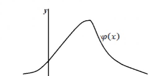
The distribution curve is a graph of the $\varphi \left(x\right)$ function of the distribution density of a random variable (Fig. 1).

Figure 2. Density distribution plot.
Geometric meaning 1: The probability of a continuous random variable falling into the interval $(\alpha ,\beta)$ is equal to the area of the curvilinear trapezoid bounded by the graph of the distribution function $\varphi \left(x\right)$ and the straight lines $x=\alpha ,$ $x=\beta $ and $y=0$ (Fig. 2).

Figure 3. Geometric representation of the probability of a continuous random variable falling into the interval $(\alpha ,\beta)$.
Geometric meaning 2: The area of an infinite curvilinear trapezoid bounded by the graph of the distribution function $\varphi \left(x\right)$, the line $y=0$ and the line variable $x$ is nothing more than the distribution function $F(x)$ (Fig. 3 ).

Figure 4. Geometric representation of the probability function $F(x)$ through the distribution density $\varphi \left(x\right)$.
Example 1
Let the distribution function $F(x)$ of a random variable $X$ have the following form.
1. Probability density of a continuous random variable
The distribution function of a continuous random variable is its comprehensive probabilistic characteristic. But it has the disadvantage that it is difficult to judge from it the nature of the distribution of a random variable in a small neighborhood of one or another point on the numerical axis. A more visual representation of the nature of the distribution of a continuous random variable in the vicinity of various points is given by a function called the probability distribution density or the differential distribution law of a random variable. In this question we will consider the probability density function and its properties.
Let there be a continuous random variable X with distribution function. Let us calculate the probability of this random variable falling into an elementary area  :
:
Let us compare this probability to the length of the section  :
:
The resulting relation is called average probability, which is per unit length of this section.
Considering the distribution function F(X) differentiable, let us pass in equality (1) to the limit at  ; then we get:
Limit of the ratio of the probability of a continuous random variable falling on an elementary section from x to x+∆x to the length of this section ∆x, when ∆х tends to zero, is called the distribution density of the random variable at point x and is denotedf (x).
By virtue of equality (2), the distribution density f(X) equal to the derivative of the distribution function F(X), i.e.
 .
.
The meaning of distribution density f(X) is that it indicates how often a random variable appears X in some neighborhood of the point X when repeating experiments.
Curve depicting distribution density f(X) random variable is called distribution curve. An approximate view of the distribution curve is presented in Fig. 1.

Note that if the possible values of a random variable fill a certain finite interval, then the distribution density f(x) = 0 outside this interval.
Let us select an elementary section ∆ on the abscissa axis X, adjacent to the point X(Fig. 2), and find the probability of hitting a random variable X
to this area. On the one hand, this probability is equal to the increment  distribution functions F(X), corresponding increment ∆
x=
dx
argument X. WITH on the other hand, the probability of a random variable hitting X
to an elementary plot dxWith accuracy up to infinitesimals of higher order than ∆ X equal to f(x)
dx
(because ∆
F(x)≈
dF(x) =f
(x)
dx).
Geometrically, this is the area of an elementary rectangle with height f(x)
and the basis dx
(Fig. 2). Magnitude f
(x)
dx
called element of probability...
distribution functions F(X), corresponding increment ∆
x=
dx
argument X. WITH on the other hand, the probability of a random variable hitting X
to an elementary plot dxWith accuracy up to infinitesimals of higher order than ∆ X equal to f(x)
dx
(because ∆
F(x)≈
dF(x) =f
(x)
dx).
Geometrically, this is the area of an elementary rectangle with height f(x)
and the basis dx
(Fig. 2). Magnitude f
(x)
dx
called element of probability...

It should be noted that not all random variables whose possible values continuously fill a certain interval are continuous random variables. There are such random variables, the possible values of which continuously fill a certain interval, but for which the distribution function is not continuous everywhere, but has discontinuities at certain points. Such random variables are called mixed. For example, in the problem of detecting a signal in noise, the amplitude of the useful signal is a mixed random variable X, which can take any value, both positive and negative.
Let us now give a more rigorous definition of a continuous random variable.
Random valueXis called continuous if its distribution functionF(x\ is continuous along the entire Ox axis, and the distribution densityf (x) exists everywhere, except perhaps for a finite number of points.
Let's consider the properties of the distribution density.
Property 1.The distribution density is non-negative, i.e. 
This property directly follows from the fact that the distribution density  is the derivative of the non-decreasing distribution function F(x).
Property 2. The distribution function of a random variable is equal to the integral of the density in the interval from – ∞ to x, i.e.
 .
(3)
.
(3)
Property 3.Probability of hitting a continuous random variableXto the site  equal to the integral of the distribution density taken over this section, i.e.
 .
(4)
.
(4)
Property 4. The integral over infinite limits of the distribution density is equal to unity:
 .
.
If the interval of possible values of a random variable has finite limits A And b,
then the distribution density f(X)= 0 outside the gap
 and property 4 can then be written as follows:
 .
.
Example. Random value X is subject to the distribution law with density
 .
.
Required:
1) Find the coefficient A.
2) Find the probability of a random variable falling into the area from 0 to .
Solution. 1) To determine the coefficient A Let's use property 4 of the distribution density:
 ,
,
where  .
.
2) According to formula (4) we have:
 .
.
Fashion  continuous random variable X its value at which the distribution density is maximum is called.
Median  continuous random variable X is a value for which it is equally probable that the random variable will be less or greater
  , that is:
Geometrically, the mode is the abscissa of the point of the distribution curve whose ordinate is maximum (for a discrete random variable, the mode is the abscissa of the polygon point with the maximum ordinate).
Geometrically, the median is the abscissa of the point at which the area limited by the distribution curve is divided in half.
Note that if the distribution is unimodal and symmetric, then the mathematical expectation, mode and median are the same.
Note also that the third central moment  or asymmetry serves as a characteristic of the “skewness” of the distribution. If the distribution is symmetrical with respect to the mathematical expectation, then for the distribution curve (histogram)
  . Fourth central point
  serves for characteristics of peaked or flat-topped distribution. These distribution properties are described using the so-called excess. We discussed the formulas for finding asymmetry and kurtosis in the previous lecture.
2.Normal distribution
Among the distributions of continuous random variables, the central place is occupied by the normal law or the Gaussian distribution law, the probability density of which has the form:
 ,
(5)
,
(5)
Where  – parameters of normal distribution.
Since the normal distribution depends on two parameters  And
And  , then it is also called two-parameter distribution.
The normal distribution law applies in cases where the random variable X is the result of a large number of different factors. Each factor separately is worth X influences insignificantly and it is impossible to indicate which one is more significant than the others. Examples of random variables that have a normal distribution include: deviation of the actual dimensions of parts processed on a machine from the nominal dimensions, errors in measurement, deviations during shooting, and others.
Let us prove that in formula (5) the parameter A is the mathematical expectation, and the parameter  – standard deviation:

 .
.
The first of the integrals is equal to zero, since the integrand is odd. The second integral is known as the Poisson integral:
 .
.
Let's calculate the variance:
 .
.
The probability density graph of a normal distribution is called a normal Gaussian curve (Fig. 3).

Let us note some properties of the curve:
1.The probability density function is defined on the entire numerical axis, that is  .
.
2. Function range  , that is, the Gaussian curve is located above the x-axis and does not intersect it.
3. The branches of the Gaussian curve asymptotically tend to the axis  , that is
4.The curve is symmetrical about the straight line  . Thus, for a normal distribution, the mathematical expectation coincides with the mode and median of the distribution.
5.The function has one maximum at the abscissa point  , equal
  . With increasing
  the Gaussian curve becomes flatter, and as it decreases
  – more “pointed”.
6. The Gaussian curve has two inflection points with coordinates  And
And  .
.
7.If, with unchanged  change the mathematical expectation, then the Gaussian curve will shift along the axis
  : to the right – when increasing A, and to the left – when decreasing.
8. Skewness and kurtosis for a normal distribution are zero.
Let's find the probability of a random variable distributed according to the normal law falling into the area  . It is known that
 .
.
 .
.
Using variable replacement
 ,
,
 .
(6)
.
(6)
Integral  is not expressed through elementary functions, therefore, to calculate the integral (6) they use tables of values of a special function, which is called Laplace function, and has the form:
 .
.
After simple transformations, we obtain a formula for the probability of a random variable falling within a given interval  :
:
 .
(7)
.
(7)
The Laplace function has the following properties:
1. .
.
2. is an odd function.
3.
 .
.
The distribution function graph is shown in Fig. 4.

Let it be necessary to calculate the probability that the deviation of a normally distributed random variable X in absolute value does not exceed a given positive number  , that is, the probability of the inequality
  .
.
Let us use formula (7) and the odd property of the Laplace function:
 .
.
Let's put  and choose
  . Then we get:
 .
.
This means that for a normally distributed random variable with parameters A And  fulfillment of inequality
  is an almost certain event. This is the so-called “three sigma” rule.
Definition . Continuous called a random variable that can take all values from some finite or infinite interval.
For a continuous random variable, the concept of distribution function is introduced.
Definition. Distribution function probabilities of a random variable X is a function F(x), which determines for each value x the probability that the random variable X will take a value less than x, that is:
F(x) = P(X< x)
Often, instead of the term “distribution function,” the term “cumulative distribution function” is used.
Properties of the distribution function:
1. The values of the distribution function belong to the segment:
0 ≤ F(x) ≤ 1.
2. The distribution function is a non-decreasing function, that is:
if x > x,
then F(x) ≥ F(x).
3. The probability that a random variable will take a value contained in the interval. The probability of such an event
P(X ≤ X ≤ X + Δ X) = F(X+ Δ X) – F(X),
those. equal to the increment of the distribution function F(X) in this area. Then the probability per unit length, i.e. average probability density in the area from X before X+ Δ X, is equal
Moving to the limit Δ X→ 0, we obtain the probability density at the point X:
representing the derivative of the distribution function F(X). Recall that for a continuous random variable F(X) is a differentiable function.
Definition. Probability density (distribution density ) f(x) of a continuous random variable X is the derivative of its distribution function
| f(x) = F′( x). | (4.8) |
About a random variable X they say that it has a distribution with density f(x) on a certain section of the x-axis.
Probability Density f(x), as well as the distribution function F(x) is one of the forms of the distribution law. But unlike the distribution function, it exists only for continuous random variables.
The probability density is sometimes called differential function or differential distribution law. The probability density plot is called distribution curve.
Example 4.4. Based on the data in Example 4.3, find the probability density of the random variable X.
Solution. We will find the probability density of a random variable as a derivative of its distribution function f(x) = F"(x).
 ◄
◄
Let us note the properties of the probability density of a continuous random variable.
1. Probability density is a non-negative function, i.e.
Geometrically, the probability of falling into the interval [ α , β ,] is equal to the area of the figure bounded from above by the distribution curve and based on the segment [ α , β ,] (Fig. 4.4).


Rice. 4.4 Fig. 4.5
3. The distribution function of a continuous random variable can be expressed in terms of the probability density according to the formula:
Geometrically properties 1 And 4 probability density means that its graph - the distribution curve - lies not below the abscissa axis, and the total area of the figure bounded by the distribution curve and the abscissa axis is equal to one.
Example 4.5. Function f(x) is given in the form:

Find: a) value A; b) expression of the distribution function F(X); c) the probability that the random variable X will take a value on the interval .
Solution. a) In order to f(x) was the probability density of some random variable X, it must be non-negative, therefore the value must be non-negative A. Given the property 4 we find:
![]() , where A = .
, where A = .
b) We find the distribution function using the property 3 :
If x≤ 0, then f(x) = 0 and, therefore, F(x) = 0.
If 0< x≤ 2, then f(x) = X/2 and therefore
If X> 2, then f(x) = 0 and therefore
c) The probability that the random variable X will take a value on the segment, we find it using the property 2 .
The definitions of the Distribution Function of a Random Variable and the Probability Density of a Continuous Random Variable are given. These concepts are actively used in articles about website statistics. Examples of calculating the Distribution Function and Probability Density using MS EXCEL functions are considered..
Let us introduce the basic concepts of statistics, without which it is impossible to explain more complex concepts.
Population and random variable
Let us have population(population) of N objects, each of which has a certain value of some numerical characteristic X.
An example of a general population (GS) is a set of weights of similar parts that are produced by a machine.
Since in mathematical statistics, any conclusion is made only on the basis of the characteristics of X (abstracting from the objects themselves), then from this point of view population represents N numbers, among which, in the general case, there may be identical ones.
In our example, GS is simply a numeric array of part weight values. X is the weight of one of the parts.
If from a given GS we randomly select one object having characteristic X, then the value of X is random variable. By definition, any random value It has distribution function, which is usually denoted F(x).
Distribution function
Distribution function probabilities random variable X is a function F(x), the value of which at point x is equal to the probability of event X F(x) = P(X Let us explain using our machine as an example. Although our machine is supposed to produce only one type of part, it is obvious that the weight of the parts produced will be slightly different from each other. This is possible due to the fact that different materials could be used in manufacturing, and the processing conditions could also vary slightly, etc. Let the heaviest part produced by the machine weigh 200 g, and the lightest - 190 g. The probability that by chance the selected part X will weigh less than 200 g is equal to 1. The probability that it will weigh less than 190 g is equal to 0. Intermediate values are determined by the form of the Distribution Function. For example, if the process is set up to produce parts weighing 195 g, then it is reasonable to assume that the probability of selecting a part lighter than 195 g is 0.5. Typical graph Distribution functions for a continuous random variable is shown in the picture below (purple curve, see example file): In MS EXCEL help Distribution function called Integral distribution function (CumulativeDistributionFunction,
CDF). Here are some properties Distribution functions: Let us remind you that distribution density is derived from distribution functions, i.e. the “speed” of its change: p(x)=(F(x2)-F(x1))/Dx with Dx tending to 0, where Dx=x2-x1. Those. the fact that distribution density>1 only means that the distribution function is growing quite quickly (this is obvious in the example). Note: The area entirely contained under the entire curve representing distribution density, is equal to 1. Note: Recall that the distribution function F(x) is called in MS EXCEL functions cumulative distribution function. This term is present in function parameters, for example NORM.DIST (x; average; standard_deviation; integral). If the MS EXCEL function should return distribution function, then the parameter integral, d.b. set to TRUE. If you need to calculate probability density, then the parameter integral, d.b. LIE. Note: For discrete distribution The probability of a random variable taking on a certain value is also often called probability density (pmf). In MS EXCEL help probability density can even be called a “probability measure function” (see the BINOM.DIST() function). It is clear that in order to calculate probability density for a certain value of a random variable, you need to know its distribution. We'll find probability density for N(0;1) at x=2. To do this, you need to write the formula =NORMAL.ST.DIST(2,FALSE)=0.054 or =NORMAL.DIST(2,0,1,FALSE). Let us remind you that probability that continuous random variable will take a specific value x is 0. For continuous random variable X can only be calculated by the probability of the event that X will take the value contained in the interval (a; b). 1) Let's find the probability that a random variable distributed by (see picture above) takes a positive value. According to property Distribution functions the probability is F(+∞)-F(0)=1-0.5=0.5. NORM.ST.DIST(9.999E+307,TRUE) -NORM.ST.DIST(0,TRUE) =1-0,5. 2) Find the probability that a random variable distributed over , took a negative value. According to the definition Distribution functions the probability is F(0)=0.5. In MS EXCEL, to find this probability, use the formula =NORMAL.ST.DIST(0,TRUE) =0,5. 3) Find the probability that a random variable distributed over standard normal distribution, will take the value contained in the interval (0; 1). The probability is equal to F(1)-F(0), i.e. from the probability of choosing X from the interval (-∞;1), you need to subtract the probability of choosing X from the interval (-∞;0). In MS EXCEL use the formula =NORM.ST.DIST(1,TRUE) - NORM.ST.DIST(0,TRUE). All calculations given above refer to a random variable distributed over standard normal law N(0;1). It is clear that the probability values depend on the specific distribution. In the distribution function article, find the point for which F(x) = 0.5, and then find the abscissa of this point. Abscissa of point =0, i.e. the probability that the random variable X will take the value<0, равна 0,5. In MS EXCEL, use the formula =NORM.ST.REV(0.5) =0. Unambiguously calculate the value random variable allows the property of monotonicity distribution functions. Inverse distribution function calculates , which are used, for example, when . Those. in our case, the number 0 is the 0.5 quantile normal distribution. In the example file you can calculate another quantile this distribution. For example, the 0.8 quantile is 0.84. In English literature inverse distribution function often referred to as Percent Point Function (PPF). Note: When calculating quantiles in MS EXCEL the following functions are used: NORM.ST.INV(), LOGNORM.INV(), CHI2.INR(), GAMMA.INR(), etc. You can read more about the distributions presented in MS EXCEL in the article.Calculation of probability density using MS EXCEL functions
Calculating probabilities using MS EXCEL functions
Instead of +∞, the value entered into the formula is 9.999E+307= 9.999*10^307, which is the maximum number that can be entered into a MS EXCEL cell (closest to +∞, so to speak).