– calculating the center of gravity of a flat bounded figure. Many readers intuitively understand what the center of gravity is, but, nevertheless, I recommend repeating the material from one of the lessons analytical geometry, where I made out problem about the center of gravity of a triangle and deciphered it in an accessible form physical meaning this term.
In independent and test assignments for the solution, as a rule, the simplest case is proposed - a flat bounded homogeneous figure, that is, a constant figure physical density– glass, wood, tin, cast iron toys, difficult childhood, etc. Further, by default, we will talk only about such figures =)
The first rule and simplest example : if a flat figure has center of symmetry, then it is the center of gravity of this figure. For example, the center of a round homogeneous plate. It is logical and understandable in everyday life - the mass of such a figure is “fairly distributed in all directions” relative to the center. I don’t want to turn it around.
However, in harsh realities, they are unlikely to throw you a sweet elliptical chocolate bar, so you’ll have to arm yourself with some serious kitchen tools:
The coordinates of the center of gravity of a flat homogeneous limited figure are calculated using the following formulas :
 , or:
, or:
 , where is the area of the region (figure); or very briefly:
![]() , Where
, Where
We will conventionally call the integral the “X” integral, and the integral the “Y” integral.
Help note
: for flat limited heterogeneous figures, the density of which is specified by the function, the formulas are more complex: , Where
 ![]() – mass of the figure;in the case of uniform density, they are simplified to the above formulas.
– mass of the figure;in the case of uniform density, they are simplified to the above formulas.
In fact, all the novelty ends with the formulas, the rest is your skill solve double integrals By the way, now is a great opportunity to practice and improve your technique. And, as you know, there is no limit to perfection =)
Let's throw in an invigorating portion of parabolas:
Example 1
Find the coordinates of the center of gravity of a homogeneous flat figure bounded by lines.
Solution: the lines here are elementary: it defines the x-axis, and the equation – a parabola, which can be easily and quickly constructed using geometric transformations of graphs:
– parabola, shifted 2 units to the left and 1 unit down.
I will complete the entire drawing at once with the finished point of the center of gravity of the figure: 
Rule two: if the figure has axis of symmetry, then the center of gravity of this figure necessarily lies on this axis.
In our case, the figure is symmetrical with respect to straight, that is, in fact, we already know the “x” coordinate of the point “em”.
Also note that vertically the center of gravity is shifted closer to the x-axis, since the figure is more massive there.
Yes, perhaps not everyone has yet fully understood what the center of gravity is: please raise your index finger up and mentally place the shaded “sole” with a dot on it. Theoretically, the figure should not fall.
We find the coordinates of the center of gravity of the figure using the formulas ![]() , Where .
, Where .
The order of traversing the area (figure) is obvious here: ![]()
Attention! Deciding on the most advantageous traversal order once- and use it for all integrals!
1) First, calculate the area of the figure. Due to the relative simplicity of the integral, the solution can be written compactly; the main thing is not to get confused in the calculations:

We look at the drawing and estimate the area by cells. It turned out to be about the case.
2) The X coordinate of the center of gravity has already been found “ graphical method", so you can refer to symmetry and move on to the next point. However, I still don’t recommend doing this - there is a high probability that the solution will be rejected with the wording “use the formula.”

Please note that here you can only get by with mental calculations - sometimes it is not at all necessary to reduce fractions to common denominator or torment the calculator.
Thus:  , which is what was required to be obtained.
3) Find the ordinate of the center of gravity. Let us calculate the “game” integral:

But here it would be hard without a calculator. Just in case, I’ll comment that as a result of multiplying polynomials, 9 terms are obtained, and some of them are similar. I gave similar terms orally (as is usually done in similar cases) and immediately wrote down the total amount.
As a result:  , which is very, very similar to the truth.
On final stage mark a point on the drawing. According to the condition, there was no requirement to draw anything, but in most tasks we are forced, willy-nilly, to draw a figure. But there is an absolute plus - a visual and quite effective verification of the result.
Answer: ![]()
The following two examples are for you to solve on your own.
Example 2
Find the coordinates of the center of gravity of a homogeneous flat figure bounded by lines ![]()
By the way, if you imagine how the parabola is located and see the points at which it intersects the axis, then here you can actually do without a drawing.
And more complicated:
Example 3
Find the center of gravity of a homogeneous flat figure bounded by lines
If you have any difficulties constructing graphs, study (repeat) lesson about parabolas and/or Example No. 11 of the article Double integrals for dummies.
Sample solutions at the end of the lesson.
In addition, a dozen or two similar examples can be found in the corresponding archive on the page Ready-made solutions for higher mathematics.
Well, I can’t help but please fans of higher mathematics, who often ask me to analyze difficult problems:
Example 4
Find the center of gravity of a homogeneous flat figure bounded by lines. Draw the figure and its center of gravity on the drawing.
Solution: the condition of this task already categorically requires the completion of the drawing. But the requirement is not so formal! – even a person with an average level of training can imagine this figure in his mind: 
A straight line cuts a circle into 2 parts, and an additional clause (cm. linear inequalities)
indicates that we are talking about a small shaded piece.
The figure is symmetrical relative to a straight line (depicted by a dotted line), so the center of gravity should lie on this line. And, obviously, its coordinates are equal modulo. An excellent guideline that virtually eliminates the possibility of an erroneous answer!
Now the bad news =) An unpleasant integral of the root is looming on the horizon, which we examined in detail in Example No. 4 of the lesson Efficient methods for solving integrals. And who knows what else will be drawn there. It would seem that due to the presence circle profitable, but not everything is so simple. The equation of the straight line is transformed to the form ![]() and the integrals will also not turn out to be sugar (although fans trigonometric integrals will appreciate). In this regard, it is more careful to dwell on Cartesian coordinates Oh.
and the integrals will also not turn out to be sugar (although fans trigonometric integrals will appreciate). In this regard, it is more careful to dwell on Cartesian coordinates Oh.
The order of traversing the figure: ![]()
1) Calculate the area of the figure:

It is more rational to take the first integral subsuming the differential sign:
And in the second integral we make the standard replacement:
![]()
Let's calculate the new limits of integration: 
2) Let's find .

Here in the 2nd integral it was again used method of subsuming a function under the differential sign. Practice and adopt these optimal (in my opinion) techniques for solving standard integrals.

After difficult and time-consuming calculations, we again turn our attention to the drawing (remember that points we don't know yet! ) and we receive deep moral satisfaction from the found value.
3) Based on the analysis carried out earlier, it remains to make sure that .

Great: 
Let's draw a point ![]() on the drawing. In accordance with the wording of the condition, we write it down as final answer:
on the drawing. In accordance with the wording of the condition, we write it down as final answer: ![]()
A similar task for you to solve on your own:
Example 5
Find the center of gravity of a homogeneous flat figure bounded by lines. Execute the drawing.
This problem is of interest because it contains a figure of a fairly small size, and if you make a mistake somewhere, then there is a high probability of “not getting into” the area at all. Which is certainly good from the point of view of decision control.
A sample design at the end of the lesson.
Sometimes it makes sense transition to polar coordinates in double integrals. It depends on the figure. I searched and searched for a successful example, but couldn’t find it, so I’ll demonstrate the solution in the 1st demo problem of the above lesson: 
Let me remind you that in that example we went to polar coordinates, found out the order of traversing the area ![]() and calculated its area
and calculated its area
Let's find the center of gravity of this figure. The scheme is the same: ![]() . The value is viewed directly from the drawing, and the “x” coordinate should be shifted a little closer to the ordinate axis, since the more massive part of the semicircle is located there.
. The value is viewed directly from the drawing, and the “x” coordinate should be shifted a little closer to the ordinate axis, since the more massive part of the semicircle is located there.
In integrals we use standard transition formulas:

Plausibly, most likely, they were not mistaken.
Lecture 4. Center of gravity.
This lecture covers the following issues
1. Center of gravity solid.
2. Coordinates of the centers of gravity of inhomogeneous bodies.
3. Coordinates of the centers of gravity of homogeneous bodies.
4. Methods for determining the coordinates of centers of gravity.
5. Centers of gravity of some homogeneous bodies.
The study of these issues is necessary in the future to study the dynamics of the movement of bodies taking into account sliding and rolling friction, the dynamics of the movement of the center of mass of a mechanical system, kinetic moments, to solve problems in the discipline “Strength of Materials”.
Bringing parallel forces.
After we have considered bringing a flat system and an arbitrary spatial system of forces to the center, we again return to considering the special case of a system of parallel forces.
Bringing two parallel forces.
In the course of considering such a system of forces, the following three cases of reduction are possible.
1. System of two collinear forces. Let us consider a system of two parallel forces directed in one direction P And Q, applied at points A And IN. We will assume that the forces are perpendicular to this segment (Fig. 1, A).
WITH, belonging to the segment AB and satisfying the condition:
AC/NE = Q/P.(1)
Main vector of the system R C = P + Q is equal in modulus to the sum of these forces: R C = P + Q.
WITH taking into account (1) is equal to zero:MC = P ∙ AC- Q∙ CB = 0.
Thus, as a result of the casting we got: R C ≠ 0, MC= 0. This means that the main vector is equivalent to the resultant passing through the center of reduction, that is:
The resultant of collinear forces is equal in modulus to their sum, and its line of action divides the segment connecting the points of their application, in inverse proportion to the moduli of these forces in an internal manner.
Note that the position of the point WITH will not change if the forces R And Q turn an angleα. Dot WITH, which has this property is called center of parallel forces.
2. System of two anticollinear and forces not equal in magnitude. May the strength P And Q, applied at points A And IN, parallel, directed in opposite directions and unequal in magnitude (Fig. 1, b).
Let us choose a point as the reduction center WITH, which still satisfies relation (1) and lies on the same line, but outside the segment AB.
The main vector of this system R C = P + Q the modulus will now be equal to the difference between the moduli of the vectors: R C = Q - P.
The main point regarding the center WITH is still zero:MC = P ∙ AC- Q∙ NE= 0, so
Resultant anticollinear and forces that are not equal in magnitude are equal to their difference, directed towards the greater force, and its line of action divides the segment connecting the points of their application, in inverse proportion to the external moduli of these forces.
Fig.1
3. System of two anticollinear and forces equal in magnitude. Let's take the previous case of reduction as the initial one. Let's fix the force R, and strength Q let us direct the modulus to the force R.
Then at Q → R in formula (1) the relation AC/NE → 1. This means that AC → NE, that is, the distance AC →∞ .
In this case, the module of the main vector R C → 0, and the modulus of the main moment does not depend on the position of the center of reduction and remains equal to the original value:
MC = P ∙ AC- Q∙ NE = P ∙ ( AC- NE) =P ∙ AB.
So, in the limit we have obtained a system of forces for which R C = 0, MC≠ 0, and the center of reduction is removed to infinity, which cannot be replaced by the resultant. It is not difficult to recognize a couple of forces in this system, so a pair of forces has no resultant.
Center of the system of parallel forces.
Consider the system n strength P i, applied at pointsA i (x i , y i , z i) and parallel to the axisOv with orth l(Fig. 2).
If we exclude in advance the case of a system equivalent to a pair of forces, it is not difficult, based on the previous paragraph, to prove the existence of its resultantR.
Let's determine the coordinates of the centerC(x c, y c, z c) parallel forces, that is, the coordinates of the point of application of the resultant of this system.
For this purpose, we use Varignon’s theorem, based on which:
M0 (R) = Σ M0(P i).

Fig.2
The vector-moment of a force can be represented as a vector product, therefore:
M 0 (R) = r c× R = Σ M0i(P i) = Σ ( r i× P i ).
Considering that R = Rv ∙ l, A P i = Pvi ∙ l and using the properties vector product, we get:
r c × Rv ∙ l = Σ ( r i × Pvi ∙ l),
r c ∙ R v× l = Σ ( r i ∙ Pvi × l) = Σ ( r i ∙ Pvi ) × l,
or:
[ r c R v - Σ ( r i Pvi )] × l= 0.
The last expression is valid only if the expression in square brackets is equal to zero. Therefore, omitting the indexvand taking into account that the resultantR = Σ P i , from here we get:
r c = (Σ P i r i )/(Σ P i ).
Projecting the last vector equality on the coordinate axis, we obtain the required expression for the coordinates of the center of parallel forces:
x c = (Σ P i x i)/(Σ P i );
y c = (Σ P i y i )/(Σ P i );(2)
z c = (Σ P i z i )/(Σ P i ).
Center of gravity of bodies.
Coordinates of the centers of gravity of a homogeneous body.
Consider a rigid body weighing P and volume V in the coordinate system Oxyz, where are the axes x And y connected to the surface of the earth, and the axis z aimed at the zenith.
If we break the body into elementary parts with a volume∆ V i , then the force of attraction will act on each part of it∆ P i, directed towards the center of the Earth. Let us assume that the dimensions of the body are significantly smaller than the dimensions of the Earth, then the system of forces applied to the elementary parts of the body can be considered not converging, but parallel (Fig. 3), and all the conclusions of the previous chapter are applicable to it.

Fig.3
Definition . The center of gravity of a solid body is the center of parallel forces of gravity of the elementary parts of this body.
Let us recall that specific gravity of an elementary part of the body is called the ratio of its weight∆ P i to volume ∆ V i : γ i = ∆ P i/ ∆ V i . For a homogeneous body this value is constant:γ i = γ = P/ V.
Substituting ∆ into (2) P i = γ i ∙∆ V i instead of P i, taking into account the last remark and reducing the numerator and denominator byg, we get expressions for the coordinates of the center of gravity of a homogeneous body:
x c = (Σ ∆ V i∙ x i)/(Σ ∆ V i);
y c = (Σ ∆ V i∙ y i )/(Σ ∆ V i);(3)
z c = (Σ ∆ V i∙ z i )/(Σ ∆ V i).
Several theorems are useful in determining the center of gravity.
1) If a homogeneous body has a plane of symmetry, then its center of gravity is in this plane.
If the axes X And at located in this plane of symmetry, then for each point with coordinates. And the coordinate according to (3), will be equal to zero, because in total All members with opposite signs are destroyed in pairs. This means that the center of gravity is located in the plane of symmetry.
2) If a homogeneous body has an axis of symmetry, then the center of gravity of the body is on this axis.
Indeed, in this case, if the axiszdraw along the axis of symmetry, for each point with coordinatesyou can find a point with coordinates and coordinates and , calculated using formulas (3), will be equal to zero.
The third theorem is proved in a similar way.
3) If a homogeneous body has a center of symmetry, then the center of gravity of the body is at this point.
And a few more comments.
First. If the body can be divided into parts for which the weight and position of the center of gravity are known, then there is no need to consider each point, and in formulas (3) P i – determined as the weight of the corresponding part and– as the coordinates of its center of gravity.
Second. If the body is homogeneous, then the weight of an individual part of it, Where - specific gravity of the material from which the body is made, and V i - the volume of this part of the body. And formulas (3) will take a more convenient form. For example,
And similarly, where - volume of the whole body.
Third note. Let the body have the form of a thin plate with an area F and thickness t, lying in the plane Oxy. Substituting in (3)∆ V i =t ∙ ∆F i , we obtain the coordinates of the center of gravity of a homogeneous plate:
x c = (Σ ∆ F i∙ x i) / (Σ ∆ F i);
y c = (Σ ∆ F i∙ y i ) / (Σ ∆ F i).
z c = (Σ ∆ F i∙ z i ) / (Σ ∆ F i).
Where – coordinates of the center of gravity of individual plates;– total body area.
Fourth note. For a body in the form of a thin curved rod of length L with cross-sectional area a elementary volume∆ V i = a ∙∆ L i , That's why coordinates of the center of gravity of a thin curved rod will be equal:
x c = (Σ ∆ L i∙ x i)/(Σ ∆ L i);
y c = (Σ ∆ L i∙ y i )/(Σ ∆ L i);(4)
z c = (Σ ∆ L i∙ z i )/(Σ ∆ L i).
Where – coordinates of the center of gravityi-th section; .
Note that, according to the definition, the center of gravity is a geometric point; it can also lie outside the boundaries of a given body (for example, for a ring).
Note.
In this section of the course we do not differentiate between gravity, gravity and body weight. In reality, gravity is the difference between the gravitational force of the Earth and the centrifugal force caused by its rotation.
Coordinates of the centers of gravity of inhomogeneous bodies.
Center of gravity coordinates inhomogeneous solid(Fig.4) in the selected reference system are determined as follows:

Fig.4


Where - weight per unit volume of a body (specific gravity)
![]() - whole body weight.
- whole body weight.
non-uniform surface(Fig. 5), then the coordinates of the center of gravity in the selected reference system are determined as follows:

Fig.5

Where - weight per unit body area,
![]() - whole body weight.
- whole body weight.
If the solid is non-uniform line(Fig. 6), then the coordinates of the center of gravity in the selected reference system are determined as follows:

Fig.6


Where - weight per body length,
Whole body weight.
Methods for determining the coordinates of the center of gravity.
Based on the general formulas obtained above, it is possible to indicate specific methods determining the coordinates of the centers of gravity of bodies.
1. Symmetry. If a homogeneous body has a plane, axis or center of symmetry (Fig. 7), then its center of gravity lies, respectively, in the plane of symmetry, axis of symmetry or in the center of symmetry.

Fig.7
2. Splitting. The body breaks into final number parts (Fig. 8), for each of which the position of the center of gravity and area are known.

Fig.8
S =S 1 +S 2.
3.Negative area method. A special case of the partitioning method (Fig. 9). It applies to bodies that have cutouts if the centers of gravity of the body without the cutout and the cutout part are known. A body in the form of a plate with a cutout is represented by a combination of a solid plate (without a cutout) with an area S 1 and the area of the cut part S2.

Fig.9
S = S 1 - S 2.
4.Grouping method. It is a good complement to the last two methods. After dividing a figure into its component elements, it is convenient to combine some of them again in order to then simplify the solution by taking into account the symmetry of this group.
Centers of gravity of some homogeneous bodies.
1) Center of gravity of a circular arc. Consider the arc AB radiusR with central angle. Due to symmetry, the center of gravity of this arc lies on the axisOx(Fig. 10).

Fig.10
Let's find the coordinate according to the formula . To do this, select on the arc AB element MM ’ length, whose position is determined by the angle. Coordinate X element MM' will. Substituting these values X And d l and keeping in mind that the integral must be extended over the entire length of the arc, we obtain:
![]()
where L is the length of arc AB, equal to .
From here we finally find that the center of gravity of a circular arc lies on its axis of symmetry at a distance from the center O equal
where is the angle measured in radians.
2) Center of gravity of the triangle's area. Consider a triangle lying in the plane Oxy, the coordinates of the vertices of which are known: A i (x i,y i ), (i= 1,2,3). Breaking the triangle into narrow strips parallel to the side A 1 A 2, we come to the conclusion that the center of gravity of the triangle must belong to the median A 3 M 3 (Fig. 11).

Fig.11
Breaking a triangle into strips parallel to the side A 2 A 3, we can verify that it must lie on the median A 1 M 1 . Thus, the center of gravity of a triangle lies at the point of intersection of its medians, which, as is known, separates a third part from each median, counting from the corresponding side.
In particular, for the median A 1 M 1 we obtain, taking into account that the coordinates of the point M 1 - this is the arithmetic mean of the coordinates of the vertices A 2 and A 3 :
x c = x 1 + (2/3) ∙ (xM 1 - x 1 ) = x 1 + (2/3) ∙ [(x 2 + x 3 )/2 - x 1 ] = (x 1 + x 2 + x 3 )/3.
Thus, the coordinates of the triangle’s center of gravity are the arithmetic mean of the coordinates of its vertices:
x c =(1/3) Σ x i ; y c =(1/3) Σ y i .
3) Center of gravity of the area of a circular sector. Consider a sector of a circle with radius R with central angle 2α , located symmetrically about the axis Ox (Fig. 12) .
It's obvious that y c = 0, and the distance from the center of the circle from which this sector is cut to its center of gravity can be determined by the formula:

Fig.12
The easiest way to calculate this integral is by dividing the integration domain into elementary sectors with an angle dφ . Accurate to infinitesimals of the first order, such a sector can be replaced by a triangle with a base equal to R × dφ and height R. The area of such a triangle dF =(1/2)R 2 ∙ dφ , and its center of gravity is at a distance of 2/3 R from the vertex, therefore in (5) we put x = (2/3)R∙ cosφ. Substituting in (5) F= α R 2, we get:

Using the last formula, we calculate, in particular, the distance to the center of gravity semicircle.
Substituting α = π /2 into (2), we obtain: x c = (4 R)/(3π) ≅ 0.4 R .
Example 1.Let us determine the center of gravity of the homogeneous body shown in Fig. 13.

Fig.13
Solution.The body is homogeneous, consisting of two parts with a symmetrical shape. Coordinates of their centers of gravity:
Their volumes:
Therefore, the coordinates of the center of gravity of the body
Example 2. Let us find the center of gravity of a plate bent at a right angle. Dimensions are in the drawing (Fig. 14).

Fig.14
Solution. Coordinates of the centers of gravity:
0.
Areas:
That's why:
Example 3.
On a square sheet
cm square hole cut
cm (Fig. 15). Let's find the center of gravity of the sheet. Example 4. Find the position of the center of gravity of the plate shown in Fig. 16. Dimensions are given in centimeters.

Fig.16
Solution. Let's divide the plate into figures (Fig. 17), centers the severity of which is known.
The areas of these figures and the coordinates of their centers of gravity:
1) a rectangle with sides 30 and 40 cm,S 1 =30 ∙ 40=1200 cm 2 ; x 1=15 cm; at 1 =20 cm.
2) right triangle with a base of 50 cm and a height of 40 cm;S 2 =0,5 ∙ 50 ∙ 40= 1000 cm 2 ; X 2 =30+50/3=46.7 cm; y 2 =40/3 =13.3 cm;
3) half circle radius circle r = 20 cm;S 3 =0,5 ∙π∙ 20 2 =628 cm 2 ; X 3 =4 R /3 π =8.5 cm; at
Solution. Recall that in physics the density of a bodyρ and its specific gravitygare related by the relation:γ = ρ g , Whereg - acceleration free fall. To find the mass of such a homogeneous body, you need to multiply the density by its volume.

Fig.19
The term “linear” or “linear” density means that to determine the mass of a truss rod, the linear density must be multiplied by the length of this rod.
To solve the problem, you can use the partitioning method. Representing a given truss as a sum of 6 individual rods, we obtain:
WhereL i lengthi th truss rod, andx i , y i - coordinates of its center of gravity.
The solution to this problem can be simplified by grouping the last 5 bars of the truss. It is easy to see that they form a figure with a center of symmetry located in the middle of the fourth rod, where the center of gravity of this group of rods is located.
Thus, a given truss can be represented by a combination of only two groups of rods.
The first group consists of the first rod, for itL 1 = 4 m,x 1 = 0 m,y 1 = 2 m. The second group of rods consists of five rods, for itL 2 = 20 m,x 2 = 3 m,y 2 = 2 m.
The coordinates of the center of gravity of the truss are found using the formula:
x c = (L 1 ∙ x 1 + L 2 ∙ x 2 )/(L 1 + L 2 ) = (4∙0 + 20∙3)/24 = 5/2 m;
y c = (L 1 ∙ y 1 + L 2 ∙ y 2 )/(L 1 + L 2 ) = (4∙2 + 20∙2)/24 = 2 m.
Note that the center WITH lies on the straight line connecting WITH 1 and WITH 2 and divides the segment WITH 1 WITH 2 regarding: WITH 1 WITH/SS 2 = (x c - x 1 )/(x 2 - x c ) = L 2 / L 1 = 2,5/0,5.
Self-test questions
- What is called the center of parallel forces?
- How are the coordinates of the center of parallel forces determined?
- How to determine the center of parallel forces whose resultant is zero?
- What properties does the center of parallel forces have?
- What formulas are used to calculate the coordinates of the center of parallel forces?
- What is the center of gravity of a body called?
- Why can the gravitational forces of the Earth acting on a point on a body be taken as a system of parallel forces?
- Write down the formula for determining the position of the center of gravity of inhomogeneous and homogeneous bodies, the formula for determining the position of the center of gravity of flat sections?
- Write down the formula for determining the position of the center of gravity of simple geometric shapes: rectangle, triangle, trapezoid and half circle?
- What is called the static moment of area?
- Give an example of a body whose center of gravity is located outside the body.
- How are the properties of symmetry used in determining the centers of gravity of bodies?
- What is the essence of the method of negative weights?
- Where is the center of gravity of a circular arc located?
- What graphical construction can be used to find the center of gravity of a triangle?
- Write down the formula that determines the center of gravity of a circular sector.
- Using formulas that determine the centers of gravity of a triangle and a circular sector, derive a similar formula for a circular segment.
- What formulas are used to calculate the coordinates of the centers of gravity of homogeneous bodies, flat figures and lines?
- What is called the static moment of the area of a plane figure relative to the axis, how is it calculated and what dimension does it have?
- How to determine the position of the center of gravity of an area if the position of the centers of gravity of its individual parts is known?
- What auxiliary theorems are used to determine the position of the center of gravity?
Goal of the work – determine the center of gravity of a complex figure analytically and experimentally.
Theoretical background. Material bodies consist of elementary particles, whose position in space is determined by their coordinates. The forces of attraction of each particle to the Earth can be considered a system of parallel forces, the resultant of these forces is called the force of gravity of the body or the weight of the body. The center of gravity of a body is the point of application of gravity.
The center of gravity is geometric point, which can be located outside the body (for example, a disk with a hole, a hollow ball, etc.). Big practical significance has a definition of the center of gravity of thin flat homogeneous plates. Their thickness can usually be neglected and the center of gravity can be assumed to be located in a plane. If coordinate plane xOy is aligned with the plane of the figure, then the position of the center of gravity is determined by two coordinates:
where is the area of part of the figure, ();
– coordinates of the center of gravity of the parts of the figure, mm (cm).
| Section of a figure | A, mm 2 | X c ,mm | Yc, mm |
 | bh | b/2 | h/2 |
 | bh/2 | b/3 | h/3 |
 | R 2a | ||
| At 2α = π πR 2 /2 |
Work procedure.
Draw a figure of complex shape, consisting of 3-4 simple figures (rectangle, triangle, circle, etc.) on a scale of 1:1 and indicate its dimensions.
Draw the coordinate axes so that they cover the entire figure, break the complex figure into simple parts, determine the area and coordinates of the center of gravity of each simple figure relative to the selected coordinate system.
Calculate the coordinates of the center of gravity of the entire figure analytically. Cut out this figure from thin cardboard or plywood. Drill two holes, the edges of the holes should be smooth, and the diameter of the holes should be slightly larger than the diameter of the needle for hanging the figure.
First hang the figure at one point (hole), draw a line with a pencil that coincides with the plumb line. Repeat the same when hanging the figure at another point. The center of gravity of the figure, found experimentally, must coincide.
Determine the coordinates of the center of gravity of a thin homogeneous plate analytically. Check experimentally
Solution algorithm
1. Analytical method.
a) Draw the drawing on a scale of 1:1.
b) Break a complex figure into simple ones
c) Select and draw coordinate axes (if the figure is symmetrical, then along the axis of symmetry, otherwise along the figure’s contour)
d) Calculate the area of simple figures and the entire figure
e) Mark the position of the center of gravity of each simple figure in the drawing
f) Calculate the coordinates of the center of gravity of each figure
(x and y axis)
g) Calculate the coordinates of the center of gravity of the entire figure using the formula
h) Mark the position of the center of gravity on drawing C (
2. Experimental determination.
The correctness of the solution to the problem can be verified experimentally. Cut out this figure from thin cardboard or plywood. Drill three holes, the edges of the holes should be smooth, and the diameter of the holes should be slightly larger than the diameter of the needle for hanging the figure.
First hang the figure at one point (hole), draw a line with a pencil that coincides with the plumb line. Repeat the same when hanging the figure at other points. The value of the coordinates of the center of gravity of the figure, found when hanging the figure at two points: . The center of gravity of the figure, found experimentally, must coincide.
3. Conclusion about the position of the center of gravity during analytical and experimental determination.
Exercise
Determine the center of gravity of a flat section analytically and experimentally.
 |  |  |
 |  |  |
 |  |  |
 |  |  |
 |  |  |
 |  |  |
 |  |  |
 |  |  |
 |  |  |
 |  |  |
Execution example
Task
Determine the coordinates of the center of gravity of a thin homogeneous plate.

I Analytical method
1. The drawing is drawn to scale (dimensions are usually given in mm)
2. We break a complex figure into simple ones.
1- Rectangle
2- Triangle (rectangle)
3- Area of the semicircle (it doesn’t exist, minus sign).
We find the position of the center of gravity of simple figures of points, and

3. Draw the coordinate axes as convenient and mark the origin of coordinates.
4. Calculate the areas of simple figures and the area of the entire figure. [size in cm]
(3. no, sign -).
Area of the entire figure
5. Find the coordinate of the central point. , and in the drawing.
6. Calculate the coordinates of points C 1, C 2 and C 3
7. Calculate the coordinates of point C
8. Mark a point on the drawing
II Experienced

Coordinates of the center of gravity experimentally.
Control questions.
1. Is it possible to consider the force of gravity of a body as a resultant system of parallel forces?
2. Can the center of gravity of the entire body be located?
3. What is the essence of the experimental determination of the center of gravity of a flat figure?
4. How is the center of gravity of a complex figure consisting of several simple figures determined?
5. How should a figure of complex shape be rationally divided into simple figures when determining the center of gravity of the entire figure?
6. What sign does the area of the holes have in the formula for determining the center of gravity?
7. At the intersection of which lines of the triangle is its center of gravity located?
8. If a figure is difficult to break down into a small number of simple figures, what method of determining the center of gravity can provide the fastest answer?
“Solving complex problems”
Goal of the work: be able to solve complex problems (kinematics, dynamics)
Theoretical background: Velocity is a kinematic measure of the movement of a point, characterizing the speed of change in its position. The speed of a point is a vector characterizing the speed and direction of movement of a point in this moment time. When specifying the motion of a point by equations, the velocity projections on the Cartesian coordinate axes are equal to:
The velocity modulus of a point is determined by the formula
The direction of the speed is determined by the direction cosines:

The characteristic of the speed of change of speed is acceleration a. The acceleration of a point is equal to the time derivative of the velocity vector:
When specifying the motion of a point, the equations for the projection of acceleration onto the coordinate axes are equal to:

Acceleration module:

Full acceleration module
The tangential acceleration module is determined by the formula

The normal acceleration modulus is determined by the formula
where is the radius of curvature of the trajectory at a given point.
The direction of acceleration is determined by the direction cosines

The equation of rotational motion of a rigid body around a fixed axis has the form
Angular velocity of the body:
Sometimes angular velocity is characterized by the number of revolutions per minute and is designated by the letter . The dependence between and has the form
Angular acceleration of the body:

A force equal to the product of the mass of a given point by its acceleration and the direction in the direction directly opposite to the acceleration of the point is called the force of inertia.
Power is the work done by a force per unit time.
Basic dynamics equation for rotational motion
– the moment of inertia of the body relative to the axis of rotation, is the sum of the products of the masses of material points by the square of their distances to this axis
Exercise
A body of mass m, with the help of a cable wound on a drum of diameter d, moves up or down along an inclined plane with an angle of inclination α. Equation of body motion S=f(t), equation of drum rotation, where S is in meters; φ - in radians; t – in seconds. P and ω are, respectively, the power and angular velocity on the drum shaft at the moment of the end of acceleration or the beginning of braking. Time t 1 – acceleration time (from rest to a given speed) or braking (from a given speed to a stop). The coefficient of sliding friction between the body and the plane is –f. Neglect friction losses on the drum, as well as the mass of the drum. When solving problems, take g=10 m/s 2
| No. var | α, deg | Law of motion | For example, movement | m, kg | t 1 , s | d, m | P, kW | , rad/s | f | Def. quantities |
| S=0.8t 2 | Down | - | - | 0,20 | 4,0 | 0,20 | m,t 1 | |||
| φ=4t 2 | Down | 1,0 | 0,30 | - | - | 0,16 | P,ω | |||
| S=1.5t-t 2 | up | - | - | - | 4,5 | 0,20 | m, d | |||
| ω=15t-15t 2 | up | - | - | 0,20 | 3,0 | - | 0,14 | m,ω | ||
| S=0.5t 2 | Down | - | - | 1,76 | 0,20 | d,t 1 | ||||
| S=1.5t 2 | Down | - | 0,6 | 0,24 | 9,9 | - | 0,10 | m,ω | ||
| S=0.9t 2 | Down | - | 0,18 | - | 0,20 | P, t 1 | ||||
| φ=10t 2 | Down | - | 0,20 | 1,92 | - | 0,20 | P, t 1 | |||
| S=t-1.25t 2 | up | - | - | - | 0,25 | P,d | ||||
| φ=8t-20t 2 | up | - | 0,20 | - | - | 0,14 | P, ω |
Execution example
Problem 1(picture 1).
Solution 1. Rectilinear movement (Figure 1, a). A point moving uniformly at some point in time received a new law of motion, and after a certain period of time stopped. Determine all kinematic characteristics of the point’s movement for two cases; a) movement along a straight path; b) movement along a curved path of constant radius of curvature r=100cm
Figure 1(a).
Law of change of point speed
We find the initial speed of the point from the condition:
We find the braking time to stop from the condition:
at , from here .
Law of motion of a point during a period of uniform motion
The distance traveled by the point along the trajectory during the braking period is
Law of change in tangential acceleration of a point
whence it follows that during the period of braking the point moved equally slow, since the tangential acceleration is negative and constant in value.
Normal acceleration points on a rectilinear trajectory of motion is equal to zero, i.e. .
Solution 2. Curvilinear movement (Figure 1, b).
Figure 1(b)

In this case, compared to the case rectilinear movement All kinematic characteristics remain unchanged, with the exception of normal acceleration.
Law of change in normal acceleration of a point
Normal acceleration of a point at the initial moment of braking
The numbering of point positions on the trajectory accepted in the drawing: 1 – current position points in uniform motion before braking begins; 2 – position of the point at the moment of braking; 3 – current position of the point during the braking period; 4 – final position of the point.
Task 2.
The load (Fig. 2, a) is lifted using a drum winch. The diameter of the drum is d=0.3m, and the law of its rotation is .
The acceleration of the drum lasted until the angular velocity. Determine all kinematic characteristics of the movement of the drum and load.


Solution. Law of change in drum angular velocity. We find the initial angular velocity from the condition: ; therefore, acceleration began from a state of rest. We will find the acceleration time from the condition: . Drum rotation angle during acceleration period.
The law of change in the angular acceleration of the drum, it follows that during the acceleration period the drum rotated with uniform acceleration.
The kinematic characteristics of the load are equal to the corresponding characteristics of any point of the traction rope, and therefore point A lying on the rim of the drum (Fig. 2, b). As is known, the linear characteristics of a point of a rotating body are determined through its angular characteristics.
The distance traveled by the load during the acceleration period, . Velocity of the load at the end of acceleration.
Acceleration of cargo.
Law of cargo movement.
The distance, speed and acceleration of the load could be determined differently, through the found law of motion of the load:
Task 3. The load, moving uniformly upward along an inclined support plane, at some point in time received braking in accordance with the new law of motion ![]() , where s is in meters and t is in seconds. Mass of the load m = 100 kg, coefficient of sliding friction between the load and the plane f = 0.25. Determine the force F and power on the traction rope for two moments of time: a) uniform movement before braking begins;
, where s is in meters and t is in seconds. Mass of the load m = 100 kg, coefficient of sliding friction between the load and the plane f = 0.25. Determine the force F and power on the traction rope for two moments of time: a) uniform movement before braking begins;
b) initial moment of braking. When calculating, take g=10 m/.
Solution. We determine the kinematic characteristics of the movement of the load.
Law of change in speed of load
Initial speed of the load (at t=0)
Cargo acceleration
Since the acceleration is negative, the movement is slow.
1. Uniform movement of the load.

To determine the driving force F, we consider the equilibrium of the load, which is acted upon by a system of converging forces: the force on the cable F, the gravitational force of the load G=mg, normal reaction supporting surface N and friction force directed towards the movement of the body. According to the law of friction, . We choose the direction of the coordinate axes, as shown in the drawing, and draw up two equilibrium equations for the load:
The power on the cable before braking begins is determined by the well-known formula
Where is m/s.
2. Slow movement of cargo.

As is known, with uneven forward movement body, the system of forces acting on it in the direction of movement is not balanced. According to d'Alembert's principle (kinetostatic method), the body in this case can be considered to be in conditional equilibrium if we add to all the forces acting on it an inertial force, the vector of which is directed opposite to the acceleration vector. The acceleration vector in our case is directed opposite to the velocity vector, since the load moves slowly. We create two equilibrium equations for the load:
Power on the cable at the start of braking
Control questions.
1. How to determine numerical value and the direction of the point's velocity at the moment?
2. What characterizes the normal and tangential components of total acceleration?
3. How to move from expressing angular velocity in min -1 to expressing it in rad/s?
4. What is body weight called? Name the unit of measurement of mass
5. At what movement material point does inertial force arise? What is its numerical value and what is its direction?
6. State d'Alembert's principle
7. Does the force of inertia arise during uniform curvilinear motion of a material point?
8. What is torque?
9. How is the relationship between torque and angular velocity expressed for a given transmitted power?
10. Basic dynamics equation for rotational motion.
Practical work No. 7
"Calculation of structures for strength"
Goal of the work: determine strength, cross-sectional dimensions and permissible load
Theoretical background.
Knowing the force factors and geometric characteristics of the section during tensile (compression) deformation, we can determine the stress using the formulas. And to understand whether our part (shaft, gear, etc.) will withstand external load. It is necessary to compare this value with the permissible voltage.
So, the static strength equation
Based on it, 3 types of problems are solved:
1) strength test
2) determination of section dimensions
3) determination of permissible load
So, the equation of static stiffness
Based on it, 3 types of problems are also solved
Equation of static tensile (compressive) strength
![]()
1) First type - strength test
![]() ,
,
i.e., we solve the left-hand side and compare it with the permissible stress.
2) Second type - determination of section dimensions
![]()
from the right side the cross-sectional area
 Section circle
hence the diameter d
Rectangle section

Section square

A = a² (mm²)
Semicircle section

Sections: channel, I-beam, angle, etc.
Area values - from the table, accepted according to GOST
3) The third type is determining the permissible load;
![]()
taken to the smaller side, integer
EXERCISE
Task
A) Strength check (test calculation)
For a given beam, construct a diagram of longitudinal forces and check the strength in both sections. For timber material (steel St3) accept ![]()
![]()
| Option No. | ||||||
| 12,5 | 5,3 | - | - | |||
| 2,3 | - | - | ||||
| 4,2 | - | - |
B) Selection of section (design calculation)
For a given beam, construct a diagram of longitudinal forces and determine the cross-sectional dimensions in both sections. For timber material (steel St3) accept
| Option No. | ||
| 1,9 | 2,5 | |
| 2,8 | 1,9 | |
| 3,2 |
B) Determination of permissible longitudinal force
For a given beam, determine the permissible values of loads and ,
construct a diagram of longitudinal forces. For timber material (steel St3) accept . When solving the problem, assume that the type of loading is the same on both sections of the beam.
| Option No. | ||||
| - | - | |||
| - | - | |||
| - | - |

 Example of completing a task
Problem 1(picture 1).
Check the strength of a column made of I-profiles of a given size. For the column material (steel St3), accept the permissible tensile stresses ![]() and during compression
and during compression ![]() . In the event of overloading or significant underloading, select I-beam sizes that ensure optimal column strength.
. In the event of overloading or significant underloading, select I-beam sizes that ensure optimal column strength.
Solution.
A given beam has two sections 1, 2. The boundaries of the sections are the sections in which the external forces. Since the forces loading the beam are located along its central longitudinal axis, only one internal force factor arises in the cross sections - longitudinal force, i.e. there is tension (compression) of the beam.

To determine the longitudinal force, we use the section method. Mentally drawing a section within each section, we will discard the lower fixed part of the beam and leave it for consideration top part. In section 1, the longitudinal force is constant and equal to
The minus sign indicates that the beam is compressed in both sections.
We build a diagram of longitudinal forces. Having drawn the base (zero) line of the diagram parallel to the axis of the beam, we plot the obtained values perpendicular to it on an arbitrary scale. As you can see, the diagram turned out to be outlined by straight lines parallel to the base one.
We check the strength of the timber, i.e. We determine the design stress (for each section separately) and compare it with the permissible one. To do this, we use the compressive strength condition
![]()
where area is a geometric characteristic of the strength of the cross section. From the table of rolled steel we take:
for I-beam
for I-beam
Strength test:
The values of longitudinal forces are taken in absolute value.
The strength of the beam is ensured, however, there is a significant (more than 25%) underload, which is unacceptable due to excessive consumption of material.
From the strength condition, we determine the new dimensions of the I-beam for each section of the beam:
Hence the required area
According to the GOST table, we select I-beam No. 16, for which;
Hence the required area
According to the GOST table, we select I-beam No. 24, for which ;
With the selected I-beam sizes, underload also occurs, but it is insignificant (less than 5%)
Task No. 2.
For a beam with given cross-sectional dimensions, determine the permissible load values and . For timber material (steel St3), accept permissible tensile stresses ![]() and during compression
and during compression ![]() .
.

Solution.
The given beam has two sections 1, 2. There is tension (compression) of the beam.
Using the method of sections, we determine the longitudinal force, expressing it through the required forces and. Carrying out a section within each section, we will discard the left part of the beam and leave it for consideration right side. In section 1, the longitudinal force is constant and equal to
In section 2, the longitudinal force is also constant and equal to
The plus sign indicates that the beam is stretched in both sections.
We build a diagram of longitudinal forces. The diagram is outlined by straight lines parallel to the base one.

From the condition of tensile strength, we determine the permissible load values and having previously calculated the areas of the given cross sections:
![]()
![]()
Control questions.
1. What internal force factors arise in the section of a beam during tension and compression?
2. Write down the tensile and compressive strength conditions.
3. How are the signs of longitudinal force and normal stress assigned?
4. How will the voltage change if the cross-sectional area increases by 4 times?
5. Are the strength conditions different for tensile and compressive calculations?
6. In what units is voltage measured?
7. Which one mechanical characteristics selected as the ultimate stress for ductile and brittle materials?
8. What is the difference between limiting and permissible stress?
Practical work No. 8
“Solving problems to determine the main central moments of inertia of flat geometric figures”
Goal of the work: determine analytically the moments of inertia of flat bodies of complex shape
Theoretical background. The coordinates of the center of gravity of the section can be expressed through the static moment:
![]()
where relative to the Ox axis
relative to the Oy axis
The static moment of the area of a figure relative to an axis lying in the same plane is equal to the product of the area of the figure and the distance of its center of gravity to this axis. The static moment has a dimension. The static moment can be positive, negative or equal to zero (relative to any central axis).
The axial moment of inertia of a section is the sum of the products or integral of elementary areas taken over the entire section by the squares of their distances to a certain axis lying in the plane of the section under consideration.
Axial moment inertia is expressed in units - . The axial moment of inertia is a quantity that is always positive and not equal to zero.
The axes passing through the center of gravity of the figure are called central. The moment of inertia about the central axis is called the central moment of inertia.
The moment of inertia about any axis is equal to the center
Draw a diagram of the system and mark the center of gravity on it. If the found center of gravity is outside the object system, you received an incorrect answer. You may have measured distances from different reference points. Repeat the measurements.
- For example, if children are sitting on a swing, the center of gravity will be somewhere between the children, and not to the right or left of the swing. Also, the center of gravity will never coincide with the point where the child is sitting.
- These arguments are valid in two-dimensional space. Draw a square that will contain all the objects of the system. The center of gravity should be inside this square.
Check your math if you get a small result. If the reference point is at one end of the system, a small result places the center of gravity near the end of the system. This may be the correct answer, but in the vast majority of cases this result indicates an error. When you calculated the moments, did you multiply the corresponding weights and distances? If instead of multiplying you added the weights and distances, you would get a much smaller result.
Correct the error if you found multiple centers of gravity. Each system has only one center of gravity. If you found multiple centers of gravity, you most likely did not add up all the moments. Center of gravity equal to the ratio“total” moment to “total” weight. There is no need to divide “every” moment by “every” weight: this way you will find the position of each object.
Check the reference point if the answer differs by some integer value. In our example, the answer is 3.4 m. Let's say you got the answer 0.4 m or 1.4 m, or another number ending in ".4". This is because you did not choose the left end of the board as your starting point, but a point that is located a whole amount to the right. In fact, your answer is correct no matter which reference point you choose! Just remember: the reference point is always at position x = 0. Here's an example:
- In our example, the reference point was at the left end of the board and we found that the center of gravity was 3.4 m from this reference point.
- If you choose as a reference point a point that is located 1 m to the right from the left end of the board, you will get the answer 2.4 m. That is, the center of gravity is 2.4 m from the new reference point, which, in turn, is located 1 m from the left end of the board. Thus, the center of gravity is at a distance of 2.4 + 1 = 3.4 m from the left end of the board. It turned out to be an old answer!
- Note: when measuring distances, remember that the distances to the “left” reference point are negative, and to the “right” reference point are positive.
Measure distances in straight lines. Suppose there are two children on a swing, but one child is much taller than the other, or one child is hanging under the board rather than sitting on it. Ignore this difference and measure the distances along the straight line of the board. Measuring distances at angles will give close but not entirely accurate results.
- For the see-saw board problem, remember that the center of gravity is between the right and left ends of the board. Later, you will learn to calculate the center of gravity of more complex two-dimensional systems.
Author: Let's take a body of arbitrary shape. Is it possible to hang it on a thread so that after hanging it retains its position (i.e. does not begin to turn) when any initial orientation (Fig. 27.1)?
In other words, is there a point relative to which the sum of the moments of gravity acting on various parts of the body would be equal to zero at any body orientation in space?
Reader: Yes, I think so. This point is called center of gravity of the body.
Proof. For simplicity, let us consider a body in the form of a flat plate of arbitrary shape, arbitrarily oriented in space (Fig. 27.2). Let's take the coordinate system X 0at with the beginning at the center of mass - point WITH, Then x C = 0, at C = 0.
 Let's imagine this body as a collection large number point masses m i, the position of each of which is specified by the radius vector.
By definition, the center of mass is , and the coordinate x C = .
Since in the coordinate system we adopted x C= 0, then . Let's multiply this equality by g and we get
As can be seen from Fig. 27.2, | x i| - this is the shoulder of power. And if x i> 0, then the moment of force M i> 0, and if x j < 0, то Mj < 0, поэтому с учетом знака можно утверждать, что для любого x i the moment of force will be equal M i = m i gx i . Then equality (1) is equivalent to equality , where M i– moment of gravity. This means that with an arbitrary orientation of the body, the sum of the moments of gravity acting on the body will be equal to zero relative to its center of mass.
In order for the body we are considering to be in equilibrium, it is necessary to apply to it at the point WITH force T = mg, directed vertically upward. The moment of this force relative to the point WITH equal to zero.
Since our reasoning did not depend in any way on how exactly the body is oriented in space, we proved that the center of gravity coincides with the center of mass, which is what we needed to prove.
Problem 27.1. Find the center of gravity of a weightless rod of length l, at the ends of which two point masses are fixed T 1 and T 2 .
| T 1 T 2 l | Solution. We will look not for the center of gravity, but for the center of mass (since these are the same thing). Let's introduce the axis X(Fig. 27.3). |
| x C =? | |
Answer: at a distance from the mass T 1 .
STOP! Decide for yourself: B1–B3.
Statement 1 . If a homogeneous flat body has an axis of symmetry, the center of gravity is on this axis.
Indeed, for any point mass m i, located to the right of the symmetry axis, there is the same point mass located symmetrically relative to the first one (Fig. 27.4). In this case, the sum of the moments of forces .
Since the entire body can be represented as divided into similar pairs of points, the total moment of gravity relative to any point lying on the axis of symmetry is equal to zero, which means that the center of gravity of the body is located on this axis. This leads to an important conclusion: if a body has several axes of symmetry, then the center of gravity lies at the intersection of these axes(Fig. 27.5).
Rice. 27.5 
Statement 2. If two bodies have masses T 1 and T 2 are connected into one, then the center of gravity of such a body will lie on a straight line segment connecting the centers of gravity of the first and second bodies (Fig. 27.6).
Rice. 27.6 ![]() Rice. 27.7
Rice. 27.7
Proof. Let us position the composite body so that the segment connecting the centers of gravity of the bodies is vertical. Then the sum of the moments of gravity of the first body relative to the point WITH 1 is equal to zero, and the sum of the moments of gravity of the second body relative to the point WITH 2 is equal to zero (Fig. 27.7).
notice, that shoulder gravity of any point mass t i the same with respect to any point lying on the segment WITH 1 WITH 2, and therefore the moment of gravity relative to any point lying on the segment WITH 1 WITH 2, the same. Consequently, the gravitational force of the entire body is zero relative to any point on the segment WITH 1 WITH 2. Thus, the center of gravity of the composite body lies on the segment WITH 1 WITH 2 .
An important practical conclusion follows from Statement 2, which is clearly formulated in the form of instructions.
Instructions,
how to find the center of gravity of a solid body if it can be broken
into parts, the positions of the centers of gravity of each of which are known
1. Each part should be replaced with a mass located at the center of gravity of that part.
2. Find center of mass(and this is the same as the center of gravity) of the resulting system of point masses, choosing a convenient coordinate system X 0at, according to the formulas:
In fact, let us arrange the composite body so that the segment WITH 1 WITH 2 was horizontal, and hang it on threads at points WITH 1 and WITH 2 (Fig. 27.8, A). It is clear that the body will be in equilibrium. And this balance will not be disturbed if we replace each body with point masses T 1 and T 2 (Fig. 27.8, b).
 Rice. 27.8
STOP! Decide for yourself: C3.
Problem 27.2. At two peaks equilateral triangle balls of mass are placed T every. A ball of mass 2 is placed at the third vertex T(Fig. 27.9, A). Triangle side A. Determine the center of gravity of this system.
| T 2T A |  Rice. 27.9 Rice. 27.9 |
| x C = ? at C = ? | |
Solution. Let us introduce the coordinate system X 0at(Fig. 27.9, b). Then
![]() ,
,
 .
.
Answer: x C = A/2; ; center of gravity lies at half height AD.