The equation is also considered in two-dimensional and one-dimensional space. In two-dimensional space, Laplace's equation is written:
∂ 2 u ∂ x 2 + ∂ 2 u ∂ y 2 = 0 (\displaystyle (\frac (\partial ^(2)u)(\partial x^(2)))+(\frac (\partial ^(2 )u)(\partial y^(2)))=0)Also in n-dimensional space. In this case, the sum is equal to zero n second derivatives.
Δ = ∂ 2 ∂ x 2 + ∂ 2 ∂ y 2 + ∂ 2 ∂ z 2 + . . . (\displaystyle \Delta =(\frac (\partial ^(2))(\partial x^(2)))+(\frac (\partial ^(2))(\partial y^(2)))+ (\frac (\partial ^(2))(\partial z^(2)))+...)- Note: everything said above applies to Cartesian coordinates in flat space (whatever its dimension). When using other coordinates, the representation of the Laplace operator changes, and, accordingly, the recording of the Laplace equation changes (for example, see below). These equations are also called Laplace's equation, but to disambiguate the terminology, an indication of the coordinate system (and, if complete clarity is desired, dimension) is usually added explicitly, for example: “two-dimensional Laplace equation in polar coordinates.”
Other forms of Laplace's equation
1 r 2 ∂ ∂ r (r 2 ∂ f ∂ r) + 1 r 2 sin θ ∂ ∂ θ (sin θ ∂ f ∂ θ) + 1 r 2 sin 2 θ ∂ 2 f ∂ φ 2 = 0 ( \displaystyle (1 \over r^(2))(\partial \over \partial r)\left(r^(2)(\partial f \over \partial r)\right)+(1 \over r^( 2)\sin \theta )(\partial \over \partial \theta )\left(\sin \theta (\partial f \over \partial \theta )\right)+(1 \over r^(2)\sin ^(2)\theta )(\partial ^(2)f \over \partial \varphi ^(2))=0)
Special points r = 0 , θ = 0 , θ = π (\displaystyle r=0,\theta =0,\theta =\pi ).
1 r ∂ ∂ r (r ∂ u ∂ r) + 1 r 2 ∂ 2 u ∂ φ 2 = 0 (\displaystyle (\frac (1)(r))(\frac (\partial )(\partial r)) \left(r(\frac (\partial u)(\partial r))\right)+(\frac (1)(r^(2)))(\frac (\partial ^(2)u)(\ partial \varphi ^(2)))=0)Special point.
1 r ∂ ∂ r (r ∂ f ∂ r) + ∂ 2 f ∂ z 2 + 1 r 2 ∂ 2 f ∂ φ 2 = 0 (\displaystyle (1 \over r)(\partial \over \partial r)\ left(r(\partial f \over \partial r)\right)+(\partial ^(2)f \over \partial z^(2))+(1 \over r^(2))(\partial ^ (2)f \over \partial \varphi ^(2))=0)Singular point r = 0 (\displaystyle r=0).
Application of Laplace's equation
Laplace's equation arises in many physical problems of mechanics, thermal conductivity, electrostatics, and hydraulics. The Laplace operator is of great importance in quantum physics, in particular in the Schrödinger equation.
Solutions of Laplace's equation
Despite the fact that Laplace's equation is one of the simplest in mathematical physics, its solution faces difficulties. The numerical solution is especially difficult due to the irregularity of the functions and the presence of singularities.
Common decision
One-dimensional space
f (x) = C 1 x + C 2 (\displaystyle f(x)=C_(1)x+C_(2))Where C 1 , C 2 (\displaystyle C_(1),C_(2))- arbitrary constants.
Two-dimensional space
The Laplace equation on a two-dimensional space is satisfied by analytic functions. Analytic functions are considered in the theory of functions of a complex variable, and the class of solutions to the Laplace equation can be reduced to a function of a complex variable.
Laplace's equation for two independent variables is formulated as follows
φ x x + φ y y = 0. (\displaystyle \varphi _(xx)+\varphi _(yy)=0.)Analytical functions
If z = x + iy, And
f (z) = u (x , y) + i v (x , y) , (\displaystyle f(z)=u(x,y)+iv(x,y),)then the Cauchy-Riemann conditions are necessary and sufficient for the function f(z) was analytical:
∂ u ∂ x = ∂ v ∂ y , ∂ u ∂ y = − ∂ v ∂ x . (\displaystyle (\frac (\partial u)(\partial x))=(\frac (\partial v)(\partial y)),~(\frac (\partial u)(\partial y))=- (\frac (\partial v)(\partial x)).)Both the real and imaginary parts of analytic functions satisfy Laplace's equation. Having differentiated the conditions
Leonardo da Vinci is considered the discoverer of capillary phenomena. However, the first accurate observations of capillary phenomena on tubes and glass plates were made by Francis Hoxby in 1709).
That matter is not infinitely divisible and has an atomic or molecular structure has been the working hypothesis for most scientists since the 18th century. Towards the end of the 19th century, when a group of positivist physicists pointed out how indirect the proof of the existence of atoms was, there was little reaction to their claim, and as a result their objections were not refuted until the beginning of this century. If in retrospect the doubts seem to us unfounded, we must remember that almost everyone who then believed in the existence of atoms also firmly believed in the material existence of the electromagnetic ether, and in the first half of the 19th century. - often caloric. However, the scientists who made the greatest contributions to the theory of gases and liquids used the assumption (usually in explicit form) of a discrete structure of matter. The elementary particles of matter were called atoms, or molecules (for example, Laplace), or simply particles (Jung), but we will follow modern concepts and use the word “molecule” for the elementary particles that make up a gas, liquid or solid.
At the beginning of the 19th century. the forces that might exist between molecules were as unclear as the particles themselves. The only force about which there was no doubt was Newtonian gravity. It acts between celestial bodies and, obviously, between one such body (the Earth) and another (for example, an apple) of laboratory mass; Cavendish had recently shown that it also acts between two laboratory masses, and therefore it was assumed that it also acts between molecules. In the early work on liquids one finds the molecular masses and mass densities entering into the equations in which we now have to write the numbers of molecules and the densities of the numbers of molecules. In a pure liquid, all molecules have the same mass, so this difference does not matter. But even before 1800 it was clear that the concept of gravitational forces was not enough to explain capillary phenomena and other properties of liquids. The rise of a liquid in a glass tube is independent of the thickness of the glass (according to Hoxby, 1709), and thus only the forces exerted by the molecules in the surface layer of the glass act on the molecules in the liquid. Gravitational forces are only inversely proportional to the square of the distance and, as was known, act freely through the intermediate substance.
The nature of intermolecular forces other than gravitational forces was very unclear, but there was no shortage of speculation. The Jesuit priest Ruggero Giuseppe Boscovich believed that molecules repel at very short distances, attract at slightly larger distances, and then exhibit alternating repulsion and attraction of decreasing magnitude as the distance increases. His ideas influenced both Faraday and Kelvin in the next century, but were too complex to be of immediate use to capillarity theorists. The latter wisely settled for simple hypotheses.
Quincke (G.H. Quincke) conducted experiments to determine the greatest distance at which the action of intermolecular forces is noticeable. He found that for various substances these distances are ~ 1/20000 of a millimeter, i.e. ~ 5 · 10 -6 cm (data given according to) .
James Jurin showed that the height to which a liquid rises is determined by the top of the tube, which is above the liquid, and is independent of the shape of the bottom of the tube. He believed that the rise of the liquid occurs due to attraction from the inner cylindrical surface of the tube, to which the upper surface of the liquid adjoins. Based on this, he showed that the rise of liquid in tubes of the same substance is inversely proportional to their inner radius.
Clairaut was one of the first to show the need to take into account the attraction between the particles of the liquid itself to explain capillary phenomena. He, however, did not recognize that the distances at which these forces act are imperceptibly small.
In 1751, von Segner introduced the important idea of surface tension by analogy with the mechanical tension of a membrane in the theory of elasticity. Today, the concept of surface tension is commonplace; it is usually the starting point for studying capillary forces and surface phenomena in educational institutions.
This idea became key in the further development of the theory. Actually, this was the first step in studying the phenomenon—a phenomenological concept was introduced that describes the macroscopic behavior of the system. The second step is the derivation of phenomenological concepts and the calculation of the values of quantities based on molecular theory. This step is of great importance, since it is a test of the correctness of a particular molecular theory.
In 1802, John Leslie gave the first correct explanation for the rise of a liquid in a tube by considering the attraction between a solid body and a thin layer of liquid on its surface. He, unlike most previous researchers, did not assume that the force of this attraction is directed upward (directly to maintain fluid). On the contrary, he showed that attraction is everywhere normal to the surface of a solid body.
The direct effect of attraction is to increase the pressure in a layer of liquid in contact with a solid so that the pressure becomes higher than that inside the liquid. The result of this is that the layer tends to “spread” over the surface of a solid body, stopped only by gravitational forces. Thus, a glass tube immersed in water is wetted with water wherever it “could crawl.” As the liquid rises, it forms a column, the weight of which eventually balances the force that causes the liquid to spread.
This theory was not written in mathematical symbols and therefore could not show a quantitative relationship between the attraction of individual particles and the final result. Leslie's theory was later revised using Laplacean mathematical methods by James Ivory in an article on capillary action, under “Fluids, Elevation of,” in an appendix to the 4th edition of the Encyclopaedia Britannica, published in 1819.
2. Theories of Jung and Laplace
In 1804, Thomas Young substantiated the theory of capillary phenomena on the principle of surface tension. He also observed the constancy of the liquid contact angle of a solid surface (contact angle) and found a quantitative relationship connecting the contact angle with the surface tension coefficients of the corresponding interphase boundaries. In equilibrium, the contact line should not move along the surface of a solid, which means, said Hawksby, he was a demonstrator at the Royal Society, and his experiments influenced the content of a very lengthy essay on the primary particles of matter and the forces between them, with which Newton completed the publication of his “Optics” in 1717 of the year. cm.
Where sSV,sSL,s LV surface tension coefficients of interphase boundaries: solid - gas (vapor), solid - liquid, liquid - gas, respectively, q edge angle. This relationship is now known as Young's formula. This work still did not have the same impact on the development of science in this direction as the article by Laplace, published a few months later, had. This seems to be due to the fact that Jung avoided using mathematical notation and tried to describe everything verbally, which makes his work seem confusing and unclear. Nevertheless, he is considered today one of the founders of the quantitative theory of capillarity.
The phenomena of cohesion and adhesion, the condensation of vapor into liquid, the wetting of solids by liquids and many other simple properties of matter - all pointed to the presence of attractive forces many times stronger than gravity, but acting only at very small distances between molecules. As Laplace said, the only condition imposed on these forces that follows from observable phenomena is that they are “imperceptible at perceptible distances.”
The repulsive forces created more trouble. Their presence could not be denied - they should balance the forces of attraction and prevent the complete destruction of matter, but their nature was completely unclear. The question was complicated by the following two erroneous opinions. Firstly, it was often believed that the active repulsive force was heat (usually the opinion of supporters of the caloric theory), since (this was the argument) a liquid, when heated, first expands and then boils, so that the molecules are separated over much greater distances than in a solid body The second misconception arose from the idea, back to Newton, that the observed pressure of a gas is due to static repulsion between molecules, and not due to their collisions with the walls of the container, as Daniel Bernoulli argued in vain.
Against this background, it was natural that the first attempts to explain capillarity, or generally the cohesion of liquids, were based on the static aspects of matter. Mechanics was a well-understood theoretical branch of science; thermodynamics and kinetic theory were still in the future. In the mechanical consideration, the key assumption was the assumption of large but short-range attractive forces. Liquids at rest (whether in a capillary tube or outside it) are obviously in equilibrium, and therefore these attractive forces must be balanced by repulsive forces. Since even less could be said about them than about the forces of attraction, they were often passed over in silence, and, in the words of Rayleigh, “the forces of attraction were left to perform the inconceivable trick of balancing themselves.” Laplace was the first to satisfactorily solve this problem, believing that repulsive forces (thermal, as he admitted) can be replaced by internal pressure, which acts everywhere in an incompressible fluid. (This assumption leads at times to uncertainty in 19th-century works as to what is strictly meant by “pressure in a fluid.”) Let us give Laplace’s calculation of internal pressure. (This conclusion is closer to the conclusions of Maxwell and Rayleigh. The conclusion is given according to.)
By 1819 he was engaged in a detailed discussion of intermolecular repulsive forces, which, although still attributed to heat or caloric, had the essential property of decreasing with distance faster than attractive forces.
It must balance the cohesive forces in the fluid, and Laplace identified this with the force per unit area which resists the division of an infinite fluid body into two widely separated semi-infinite bodies bounded by flat surfaces. The derivation below is closer to that of Maxwell and Rayleigh than to Laplace's original form, but there is no significant difference in the argumentation.
Let us consider two semi-infinite liquid bodies with strictly flat surfaces, separated by a layer (thickness l) pair with negligibly low density (Fig. 1), and in each of them we select a volume element. The first is in the upper body at a height r above the flat surface of the lower body; its volume is equal dxdydz. The second is located in the lower body and has a volume where the origin of polar coordinates coincides with the position of the first elementary volume. Let f(s) is the force acting between two molecules separated by a distance s, A d- radius of its action. Since this is always an attractive force, we have
If r is the density of the number of molecules in both bodies, then the vertical component of the force of interaction between two volume elements is equal to
The total force of attraction per unit area (positive value) is

Let u(s) is the potential of intermolecular force:

Integrating by parts again, we get
![]()
Internal Laplace pressure K is the force of attraction per unit area between two flat surfaces when they come into contact, i.e. F(0):
![]()
where is a volume element, which can be written as . Because the u(r) by assumption is negative or equal to zero everywhere, then K positively. Laplace believed that K is large compared to atmospheric pressure, but the first realistic numerical estimate was to be made by Young.
The above conclusion is based on the implicit assumption that the molecules are distributed uniformly with density r, i.e. the liquid does not have a discernible structure on a size scale commensurate with the radius of action of the forces d. Without this assumption, it would be impossible to write expressions (2) and (3) in such a simple form, but it would be necessary to find out how the presence of a molecule in the first volume element affects the probability of the presence of a molecule in the second.
The tension per unit length along an arbitrary line on the surface of the liquid must be equal (in the appropriate system of units) to the work expended to create a unit of free surface area. This follows from the experiment on stretching a liquid film (Fig. 2).

The value of this work can be immediately obtained from expression (6) for F(l). If we take two semi-infinite bodies in contact and separate them to a distance exceeding the radius of action of intermolecular forces, the work per unit area will be determined as
![]() (8)
(8)
During separation, two free surfaces are formed, and therefore the work expended can be equated to twice the surface energy per unit area, which is equal to surface tension:
![]() (9)
(9)
Thus, K is the integral of the intermolecular potential, or its zero moment, and H— his first moment. While K inaccessible to direct experiment, H can be found if we can measure surface tension.
Let be the density of cohesive energy at some point in the liquid or gas, i.e. attitude dU/dV Where d U— internal energy of small volume V liquid or gas containing this point. For the molecular model we accept
![]() (10)
(10)
Where r— distance from the point in question. Rayleigh identified Laplace's K with a difference of this potential of 2 between a point on a flat surface of the liquid (value 2 S) and a dot inside (value 2 I). On the surface, integration in (10) is limited to a hemisphere of radius d, and in the internal region it is carried out throughout the entire sphere. Hence, S there is half I, or
![]() (11)
(11)
Let us now consider a drop of radius R. Calculation fI does not change, but upon receipt f S integration is now carried out over a more limited volume due to the curvature of the surface. If is the angle between the vector and a fixed radius, then
Then the internal pressure in the drop is
Where H is determined by equation (9). If we took not a spherical drop, but a portion of liquid with a surface determined by two main radii of curvature R 1 And R 2, then we would get internal pressure in the form
![]() (14)
(14)
According to Euler's theorem, the sum is equal to the sum of the inverse radii of curvature of the surface along any two orthogonal tangents.
Because K And H positive and R is positive for a convex surface, then from (13) it follows that the internal pressure in a drop is higher than in a liquid with a flat surface. On the contrary, the internal pressure in a fluid bounded by a concave spherical surface is lower than in a fluid with a flat surface, since R in this case it is negative.
These results form the basis of Laplace's theory of capillarity. Equation for the pressure difference (fluid pressure inside a spherical drop of radius R) and (gas pressure outside) is now called Laplace's equation:
Three ideas are enough - surface tension, internal pressure and contact angle, as well as expressions (1) and (15) to solve all problems of ordinary equilibrium capillarity using classical statics methods. Thus, after the work of Laplace and Young, the foundations of the quantitative theory of capillarity were laid.
Young's results were obtained later by Gauss using the variational method. But all these works (by Young, Laplace and Gauss) had one common drawback, a flaw, so to speak. This drawback will be discussed later.
When calculating the pressure inside a curved liquid surface, the Rayleigh potential 2 (10) was introduced; It was also noted in passing that I is the cohesive energy density. This useful concept was first introduced in 1869 by Dupre, who defined it as the work of crushing a piece of a substance into its constituent molecules (la travail de désagré gation totale - the work of complete disaggregation).

Inward force acting on a molecule at depth r< d , is opposite in sign to the outward force that would arise from the molecules in the shaded volume if it were filled uniformly with density.
He cites the conclusion made by his colleague F. J. D. Massier as follows. The force acting on the molecule at the surface towards the volume of the liquid is opposite in sign to the force arising from the shaded volume in Fig. 3, since inside the liquid the force of attraction from the spherical volume of radius is zero due to symmetry. Thus, the force directed inward is
This force is positive because f(0 < s < d) < 0 и F(d) = 0 due to odd function f(s). No force acts on a molecule unless it is within a distance d on one side or the other of the surface. Therefore, the work done to remove one molecule from a liquid is
because the u(r) is an even function. This work is equal to minus twice the energy per molecule required to disintegrate the liquid ( doubled, so as not to count molecules twice: once when removing them, another time as part of the environment):
![]() (18)
(18)
This is a simple and understandable expression for internal energy U liquid containing N molecules. It follows that the cohesive energy density is given by expression (10), or
which coincides with (11), if we remove the index I. Dupre himself obtained the same result in a roundabout way. He was counting dU/dV through work against intermolecular forces during the uniform expansion of a cube of liquid. It gave him
Because the K has the form ((7) and (11)), where the constant a is given by the expression
![]() (21)
(21)
then integration (20) again leads to (19).
Rayleigh criticized Dupre's conclusion. He believed that consideration of the work of uniform expansion from the state of balance of cohesive and repulsive intermolecular forces when taking into account only cohesive forces was unfounded; Before taking such a step, one should have a better knowledge of the type of repulsive forces.
We see that in this conclusion, as in the conclusions of Young, Laplace and Gauss, the assumption of an abrupt change in the density of the number of molecules of a substance at the phase interface is significantly used. At the same time, in order for the above arguments to describe real phenomena in matter, it is necessary to assume that the radius of action of intermolecular forces in matter is much greater than the characteristic distance between particles. But under this assumption, the interface between the two phases cannot be sharp—a continuous transition density profile must arise, in other words, a transition zone.
Attempts have been made to generalize these findings to a continuous transient profile. In particular, Poisson, trying to follow this path, came to the erroneous conclusion that in the presence of a transition profile, surface tension should disappear altogether. Maxwell later showed the fallacy of this conclusion.
However, the very assumption that the radius of action of intermolecular forces in a substance is much greater than the characteristic distance between particles does not correspond to experimental data. In reality, these distances are of the same order. Therefore, a mechanistic consideration in the spirit of Laplace is, in modern terms, a mean field theory. The same is the Vander Waals theory, not described here, which gave the famous equation of state of real gases. In all these cases, an accurate calculation requires taking into account correlations between particle number densities at different points. This makes the task very difficult.
3. Gibbs theory of capillarity
As often happens, the thermodynamic description turns out to be simpler and more general, not being limited by the shortcomings of specific models.
It was in this way that Gibbs described capillarity in 1878, constructing a purely thermodynamic theory. This theory became an integral part of Gibbs' thermodynamics. Gibbs' theory of capillarity, without relying directly on any mechanistic models, is devoid of the shortcomings of Laplace's theory; it can rightfully be considered the first detailed thermodynamic theory of surface phenomena.
About Gibbs' theory of capillarity we can say that it is very simple and very complex. Simple because Gibbs managed to find a method that allows us to obtain the most compact and elegant thermodynamic relations, equally applicable to flat and curved surfaces. “One of the main tasks of theoretical research in any field of knowledge,” wrote Gibbs, “is to establish that point of view from which the object of study appears with the greatest simplicity.” This point of view in Gibbs' theory of capillarity is the idea of separating surfaces. The use of a visual geometric image of the dividing surface and the introduction of redundant quantities made it possible to describe the properties of surfaces as simply as possible and to bypass the question of the structure and thickness of the surface layer, which was completely unstudied at the time of Gibbs and still remains far from completely resolved. Excess Gibbs values (adsorption and others) depend on the position of the separating surface, and the latter can also be found for reasons of maximum simplicity and convenience.
It is reasonable to choose in each case the dividing surface so that it is everywhere perpendicular to the density gradient. If separating surfaces are selected, then each phase ( l} (l = a, b, g) now corresponds to the volume it occupies V{ l) . Full system volume
Let be the density of the number of molecules of the variety j in the [bulk] phase ( l). Then the total number of molecules of the sort j in the system under consideration is equal to
![]()
where is the surface excess number of molecules of the type j(index ( s) means surface - surface). Excesses of other extensive physical quantities are determined in a similar way. Obviously, in the case of, for example, a flat film, it is proportional to its area A. The value defined as the surface excess in the number of molecules of a type j per unit area of the spreading surface is called adsorption of molecules of the type j on this surface.
Gibbs used two main positions of the separating surface: one in which the adsorption of one of the components is zero (now this surface is called equimolecular), and a position for which the obvious dependence of the surface energy on the curvature of the surface disappears (this position was called by Gibbs the tension surface). Gibbs used the equimolecular surface to consider flat liquid surfaces (and surfaces of solids), and the tension surface to consider curved surfaces. For both positions, the number of variables is reduced and maximum mathematical simplicity is achieved.
Now about the complexity of Gibbs' theory. Although very simple mathematically, it is still difficult to understand; This happens for several reasons. Firstly, Gibbs' theory of capillarity cannot be understood in isolation from the entirety of Gibbs' thermodynamics, which is based on a very general, deductive method. The great generality of a theory always gives it some abstractness, which, of course, affects the ease of perception. Secondly, Gibbs’ theory of capillarity itself is an extensive but conditional system that requires unity of perception without abstraction from its individual provisions. An amateurish approach to studying Gibbs is simply impossible. Finally, an important circumstance is that all of Gibbs’s mentioned work is written in a very concise manner and in very difficult language. This work, according to Rayleigh, is “too condensed and difficult not only for most, but, one might say, for all readers.” According to Guggenheim, "it is much easier to use Gibbs's formulas than to understand them."
Naturally, the use of Gibbs' formulas without their true understanding led to numerous errors in the interpretation and application of individual provisions of Gibbs' theory of capillarity. Many errors were associated with a lack of understanding of the need to unambiguously determine the position of the dividing surface in order to obtain the correct physical result. Errors of this kind were often encountered when analyzing the dependence of surface tension on surface curvature; Even one of the “pillars” of the theory of capillarity, Bakker, did not escape them. An example of another type of error is the incorrect interpretation of chemical potentials when considering surface phenomena and external fields.
Already soon after the publication of Gibbs' theory of capillarity, wishes were expressed for its more complete and detailed explanation in the scientific literature. In the letter to Gibbs quoted above, Rayleigh suggested that Gibbs himself take on this work. However, this was done much later: Rice prepared a commentary on Gibbs’ entire theory, and some of its provisions were commented on in the works of Frumkin, Defay, Rehbinder, Guggenheim, Tolman, Buff, Semenchenko and other researchers. Many provisions of Gibbs' theory became clearer, and simpler and more effective logical techniques were found to justify them.
A typical example is Kondo's impressive work, which proposed a visual and easy-to-understand method for introducing a tension surface by mentally moving the dividing surface. If we write an expression for the energy of an equilibrium two-phase system a - b (a- internal and b- external phase) with a spherical fracture surface
U = T.S. - P a V a- P b V b+ sA +(22)
and we will mentally change the position of the dividing surface, i.e. change its radius r, then, obviously, such physical characteristics as energy U, temperature T, entropy S, pressure R, chemical potential i th component m i and its mass m i, as well as the full volume of the system V a+ V b remains unchanged. As for the volume V a = 4 /3pr 3 and areas A = 4pr 2 and surface tension s, then these quantities will depend on the position of the dividing surface and therefore for the specified mental process of change r we get from (22)
- P a dVa+ Pb dVb + sdA + Ads = 0 (23)
![]() (24)
(24)
Equation (24) determines the nonphysical (this circumstance is marked with an asterisk) dependence of surface tension on the position of the dividing surface. This dependence is characterized by a single minimum s, which corresponds to the tension surface. Thus, according to Kondo, a tension surface is a dividing surface for which surface tension has a minimum value.
Gibbs introduced the tension surface in a different way. He proceeded from the basic equation of the theory of capillarity
(the bar above means excess for an arbitrary dividing surface with principal curvatures WITH 1 and C 2) and considered the physical (and not purely mental) process of surface curvature at a given position and fixed external conditions.
According to Gibbs, the tension surface corresponds to a position of the dividing surface in which the curvature of the surface layer, with constant external parameters, does not affect the surface energy and also corresponds to the condition:
¶ s/¶ r =0 (26)
Guggenheim comments on Gibbs's proof: "I found Gibbs's discussion difficult, and the more carefully I studied it, the more obscure it seemed to me." This recognition indicates that understanding the Gibbs tension surface has been difficult even for thermodynamicists.
As for Kondo's approach, it is clear at first glance. However, it is necessary to ensure that the Gibbs and Kondo tension surfaces are adequate. This can be demonstrated, for example, using the hydrostatic determination of surface tension
Young mentioned the presence of a density gradient in a layer of finite thickness, but discarded this effect, considering it insignificant.
Pt— local value of the tangential component of the pressure tensor;
r"— radial coordinate; radii R a And Rb limit the surface layer.
Differentiation (27) with mental movement of the dividing surface and constancy of the physical state (Kondo approach) leads to equation (24). Differentiation with curvature of the surface layer and constancy of the physical state (Gibbs approach, in this case R a And Rb variables) gives
![]() (28)
(28)
where it is taken into account that P t(P a) = P a And P t(P b) = P b.
From equations (28) and (24) it is clear that condition (26) is equivalent to condition ( d s/ dr) * = 0 and, therefore, Kondo’s simpler and more intuitive approach is adequate to Gibbs’ approach.
The introduction of the concept of a dividing surface made it possible to mathematically strictly define the previously purely intuitive concept of a phase boundary and, therefore, to use precisely defined quantities in equations. In principle, Gibbs surface thermodynamics describes a very wide range of phenomena, and therefore (apart from realizations, reformulations, more elegant derivations and proofs) very little new has been done in this field since its inception. But still, some results, mainly related to those issues that were not covered by Gibbs, must be mentioned.
This theory was not written in mathematical symbols and therefore could not show a quantitative relationship between the attraction of individual particles and the final result. Leslie's theory was later revised using Laplacean mathematical methods by James Ivory in an article on capillary action, under “Fluids, Elevation of,” in an appendix to the 4th edition of the Encyclopaedia Britannica, published in 1819.
Theories of Jung and Laplace.
In 1804, Thomas Young substantiated the theory of capillary phenomena on the principle of surface tension. He also observed the constancy of the liquid contact angle of a solid surface (contact angle) and found a quantitative relationship connecting the contact angle with the surface tension coefficients of the corresponding interphase boundaries. In equilibrium, the contact line should not move along the surface of a solid body, which means that he said
where sSV, sSL, sLV are the surface tension coefficients of the interphase boundaries: solid - gas (vapor), solid - liquid, liquid - gas, respectively, q - contact angle. This relationship is now known as Young's formula. This work still did not have the same impact on the development of science in this direction as the article by Laplace, published a few months later, had. This seems to be due to the fact that Jung avoided using mathematical notation and tried to describe everything verbally, making his work seem confusing and unclear. Nevertheless, he is considered today one of the founders of the quantitative theory of capillarity.
The phenomena of cohesion and adhesion, the condensation of vapor into liquid, the wetting of solids by liquids and many other simple properties of matter - all pointed to the presence of attractive forces many times stronger than gravity, but acting only at very small distances between molecules. As Laplace said, the only condition imposed on these forces that follows from observable phenomena is that they are “imperceptible at perceptible distances.”
The repulsive forces created more trouble. Their presence could not be denied - they must balance the forces of attraction and prevent the complete destruction of matter, but their nature was completely unclear. The question was complicated by the following two erroneous opinions. Firstly, it was often believed that the active repulsive force was heat (usually the opinion of supporters of the caloric theory), since (this was the argument) a liquid, when heated, first expands and then boils, so that the molecules are separated over much greater distances than in a solid body The second misconception arose from the idea, back to Newton, that the observed pressure of a gas is due to static repulsion between molecules, and not due to their collisions with the walls of the container, as Daniel Bernoulli argued in vain.
Against this background, it was natural that the first attempts to explain capillarity, or generally the cohesion of liquids, were based on the static aspects of matter. Mechanics was a well-understood theoretical branch of science; thermodynamics and kinetic theory were still in the future. In the mechanical consideration, the key assumption was the assumption of large but short-range attractive forces. Liquids at rest (whether in a capillary tube or outside it) are obviously in equilibrium, and therefore these attractive forces must be balanced by repulsive forces. Since even less could be said about them than about the forces of attraction, they were often passed over in silence, and, in the words of Rayleigh, “the forces of attraction were left to perform the inconceivable trick of balancing themselves.” Laplace was the first to satisfactorily solve this problem, believing that repulsive forces (thermal, as he admitted) can be replaced by internal pressure, which acts everywhere in an incompressible fluid. (This assumption leads at times to uncertainty in 19th-century works as to what is strictly meant by “pressure in a fluid.”) Let us give Laplace’s calculation of internal pressure. (This conclusion is closer to the conclusions of Maxwell and Rayleigh. The conclusion is given according to.)
It must balance the cohesive forces in the fluid, and Laplace identified this with the force per unit area which resists the division of an infinite fluid body into two widely separated semi-infinite bodies bounded by flat surfaces. The derivation below is closer to that of Maxwell and Rayleigh than to Laplace's original form, but there is no significant difference in the argumentation.
Let us consider two semi-infinite liquid bodies with strictly flat surfaces, separated by a layer (thickness l) of vapor with a negligible density (Fig. 1), and in each of them we select a volume element. The first is located in the upper body at a height r above the flat surface of the lower body; its volume is equal to dxdydz. The second is located in the lower body and has a volume ![]() , where the origin of polar coordinates coincides with the position of the first elementary volume. Let f(s) be the force acting between two molecules separated by a distance s, and let d be the radius of its action. Since this is always an attractive force, we have
, where the origin of polar coordinates coincides with the position of the first elementary volume. Let f(s) be the force acting between two molecules separated by a distance s, and let d be the radius of its action. Since this is always an attractive force, we have
If r is the density of the number of molecules in both bodies, then the vertical component of the interaction force between two volume elements is equal to
The above conclusion is based on the implicit assumption that the molecules are distributed uniformly with density r, i.e. the liquid does not have a discernible structure on a size scale commensurate with the radius of action of forces d. Without this assumption, it would be impossible to write expressions (2) and (3) in such a simple form, but it would be necessary to find out how the presence of a molecule in the first volume element affects the probability of the presence of a molecule in the second.
EXTRACTING THE CONTOUR OF A LIQUID DROPLET IN THE PROBLEM OF DETERMINING SURFACE TENSION
Mizotin M.M. 1, Krylov A.S. 1, Protsenko P.V. 2
1 Moscow State University named after M.V. Lomonosov, Faculty of Computational Mathematics and Mathematics
2 Moscow State University named after M.V. Lomonosov, Faculty of Chemistry
Introduction
Surface tension is one of the most important properties of liquids, and its accurate measurement is essential for studying various phenomena and developing technological processes. There are a number of ways to measure surface tension, but among all of them, the sessile or hanging drop method can be distinguished. The main advantages of the method are its very wide range of applications - from light fluid liquids to liquid metals, and the relative simplicity of the experimental setup compared to other methods. Moreover, due to the development of digital computing and photographic technology, it has become possible to perform analysis almost instantly.
The essence of the method is as follows: a drop is placed on a horizontal substrate (lying drop method) or suspended on a capillary tube (hanging drop method) and then its profile photograph is studied. Measuring the geometric parameters of an equilibrium drop, the shape of which is determined by the relationship between the density and surface tension of the liquid, makes it possible to restore the desired surface tension. The installation diagram is shown in Fig. 1.
Rice. 1. 1 – light source (lamp or microscope mirror), 2 – drop on the substrate,
3 – microscope with a digital camera.
Despite a fairly well-developed experimental technique, a special expensive installation for shooting a drop is still required. This paper proposes an algorithm for an experimental setup made from widely available components. The disadvantages of the installation in comparison with laboratory equipment are compensated by the proposed image processing methods.
Sessile drop method
The basic equation of the sessile drop method, the Young-Laplace equation, describes the surface of a drop with rotational symmetry on a horizontal substrate. To solve this problem, an effective technique was proposed, subsequently improved and supplemented.
This technique is based on the numerical differentiation of the Young-Laplace equation. In order to differentiate the Young-Laplace equation, a parameterization of the curve is introduced  , Where t– length of the arc of the curve from the top of the drop (Fig. 2).

Rice. 2. Parameterization of the drop contour.
This parameterization satisfies the condition  , and leads to the system of equations
 (1)
(1)
with initial conditions  ,
,  ,
,  ,
,  and additional condition
  . In the developed software package, the Cauchy problem (1) is solved by the Runge-Kutta method of the fourth order of accuracy.
To restore the parameters of a sessile drop, it is necessary to solve the inverse problem of determining the capillary constant  , coordinates of the drop apex
  and its radius of curvature
  as a function of the radius of the horizontal section of the droplet from the height above the substrate. This function is measured with error and, in some cases, measurements of only part of the drop contour are available. When solving this inverse problem, the error (2) is minimized
between experimental points  and the curve obtained as a result of the numerical solution of problem (2). The difference between the experimental points and the curve is defined as the root of the sum of the squares of the distances from each experimental point to the curve.
In this regard, the following image processing task arises: automatically obtaining the outline of a drop, which is complicated by the presence of dust and debris in the images (which is associated with the use of a conventional camera in “domestic” conditions), as well as variable lighting conditions.
Error function
One of the main parts of the method is the calculation of the error function (2). Calculate the distance between a point and a curve (3)
in this case it is very labor-intensive, since  unknown to us, and they also need to be found numerically using a one-dimensional search method.
To efficiently calculate the error function, the following algorithm is proposed. Firstly, it is necessary to sort all experimental points so that with increasing point number i
the corresponding parameter also increased. Then, when searching for a parameter for each subsequent point, you can use the parameter value as an initial approximation  , and for the first point the initial approximation will be
  . For more information on drawing the outline of a drop, see below.
Secondly, the calculation of the error function can be carried out directly during the process of integrating system (1) using the Runge-Kutta method. In fact, at each iteration the values are available to us, and the smallest distance from the point can be found by solving equation (4)
Newton's method. That is, when numerically integrating system (1), you need to monitor the value of function (4) for each subsequent point, and remember the values of the smallest errors, if necessary, reducing the step by  to increase the accuracy of the results.
Selecting the outline of a drop
As mentioned above, to effectively calculate the error using formula (4), it is necessary to extract the contour of the drop from the image in such a way that with increasing point number i the corresponding parameter also increased. This operation is carried out in 2 stages: direct selection of edges using the Canny detector and selection of related sequential sets of points from the resulting binary map of edges.
The following algorithm was developed for edge tracking. First, it is necessary to perform an edge thinning operation, since the Canny detector does not guarantee that all the resulting edges will be 1 pixel thick (this situation mainly occurs at junctions), and such a condition is necessary for further processing. Edge thinning surgery can be performed using one of the known edge thinning techniques. In this work, the algorithm was used.
Further processing is based on the analysis of a 3x3 pixel neighborhood around the pixel in question. In Fig. 3 pixel values in the neighborhood are represented by variables  , taking the value 0 or 1.

Rice. 3. 3x3 neighborhood around the pixel in question  ,
,  .
.
General scheme of the algorithm for identifying connected sequences of points:

If  And
And  , then the central pixel contains the intersection of the contours.
If  and , then the end of the contour is located in the central pixel.
At the same time, checking these conditions can be quickly and efficiently done using lookup tables, since the total possible input values are 512 = 2 9 .
Start from one of the found ends of the contours.
Add the current pixel to the list of contour pixels under the current number and mark the current pixel on the edge map with the number of the current contour.
Find a pixel with value 1 among the neighbors of the current pixel.
If the found neighbor is not the end of a contour or an intersection and is not yet marked with any numbers on the edge map, then move the current pixel to the position of the found neighbor and go to step 3. Otherwise, finish filling the current contour and go to the next one (step 2).
Conclusion
Experimental studies of the paraffin oil/decane system at various concentrations using the proposed algorithm showed the effectiveness of the proposed approach.
The work was carried out with the support of the Federal Target Program “Scientific and scientific-pedagogical personnel of innovative Russia” for 2009–2013.
Literature
Maze C., Burnet G. A Non-linear Regression Method for Calculating the Surface Tension and Contact Angle from the Shape of a Sessile Drop // Surf. Sci. 1969. V. 13. P. 451.
Krylov A. S., Vvedensky A. V., Katsnelson A. M., Tugovikov A. E.. Software package for determination of surface tension of liquid metals // J. Non-Cryst.Solids. 1993. V. 156-158. P. 845.
O. I. del Río and A. W. Neumann. Axisymmetric Drop Shape Analysis: Computational Methods for the Measurement of Interfacial Properties from the Shape and Dimensions of Pendant and Sessile Drops // Journal of Colloid and Interface Science, Volume 196, Issue 2, 15 December 1997, Pages 136-147.
M. Hoorfar and A. W. Neumann. Recent progress in Axisymmetric Drop Shape Analysis // Advances in Colloid and Interface Science, Volume 121, Issues 1-3, 13 September 2006, Pages 25-49.
Canny, J., A Computational Approach To Edge Detection // IEEE Trans. Pattern Analysis and Machine Intelligence, 8(6):679–698, 1986
Lam L., Lee S.-W., Suen C.Y. Thinning Methodologies - A Comprehensive Survey // IEEE Transactions on Pattern Analysis and Machine Intelligence archive, Volume 14 Issue 9, September 1992.
Z. Guo and R. W. Hall, “Parallel thinning with two-subiteration algorithms,” Comm. ACM, vol. 32, no. 3, pp. 359-373, 1989.
DROPLET EDGE DETECTION FOR SURFACE TENSION DETERMINATION
Mizotin M. 1, Krylov A. 1, Protsenko P. 2
1 Lomonosov Moscow State University, Faculty of Computational Mathematics and Cybernetics, Laboratory of Mathematical Methods of Image Processing,
2 Lomonosov Moscow State University, Department of Chemistry
Surface tension is one of the key propertied of liquid, thus its measurement is crucial for studying various phenomena such as wetting and development of technological processes. There sessile and pendant drop techniques are one of the most frequently used because of their universality and simplicity of measurement process.
The method is based on studying of the axisymmetric drop profile. The balance of gravity force and surface tension forms the distinct profile shape, thus surface tension can be calculated by the solution of the inverse problem for the Young-Laplace equation.
In this work the method of droplet contour extraction for determination of the surface tension is presented. The key difference of the proposed method is its orientation on inexpensive experimental setup using widely available components such as standard microscope, digital camera and substrate holder. Proposed techniques of image processing allow to avoid most of the problems concerning inferior quality of the drop images acquired by inexpensive setup retaining the measurement accuracy.
The work was supported by target federal program “Scientific and scientific-pedagogical personnel of innovative Russia in 2009-2013”.
APPLICATION OF THE METHOD OF MORPHOLOGICAL AMOEBAES FOR ISOLATION
WITHVESSELS IN FUNDUS IMAGES
Nasonov A.V. 1, Chernomorets A.A. 1, Krylov A.S. 1, Rodin A.S. 2
Moscow State University named after M.V. Lomonosov,
1 Faculty of Computational Mathematics and Cybernetics, Laboratory of Mathematical Methods of Image Processing /
2 Faculty of Fundamental Medicine, Department of Ophthalmology
The work developed an algorithm for identifying vessels in fundus images, based on the use of the method of morphological amoebae. The application of the algorithm to the problem of extending vessels from a set of points that are known to be points of vessels is considered.
1. Introduction
Fundus photographs are used to diagnose retinal diseases. Segmentation and assessment of the characteristic sizes of the vessels of the retinal circulatory system are of great interest in the diagnosis and treatment of many eye diseases.
Identification of vessels in retinal images is a rather difficult task in image processing due to high noise levels, uneven illumination, and the presence of objects similar to vessels. Among the methods for detecting vessels in fundus images, the following classes can be distinguished:
A class of methods that use image convolution with a two-dimensional directional filter and subsequent detection of response peaks. In order to segment the vascular network, a two-dimensional linear filter is proposed, the profile of which is a Gaussian. The advantage of this approach is the stable identification of straight sections of vessels and the calculation of their width. However, the method does not detect thin and tortuous vessels well; false alarms are possible for objects that are not vessels, for example, exudates.
Methods using ridge detection. Primitives are found - short segments lying in the middle of the lines, then, using machine learning methods, primitives are selected that correspond to the vessels along which the vascular tree is restored.
Methods using vessel tracking, which includes both connecting vessels at a pair of points and continuing vessels. The advantages of this approach include high accuracy of work on thin vessels and restoration of ruptured vessels. The disadvantage is the difficulty of processing branching and crossing vessels.
Pixel-by-pixel classification based on the application of machine learning methods. Here, for each pixel, a feature vector is constructed, on the basis of which it is determined whether the pixel is part of the vessel or not. To train the method, images of the fundus with vessels marked on it by an expert are used. The disadvantages of the method include the large discrepancy in expert opinions.
In this work, the method of morphological amoebas is used to identify vessels - a morphological method in which a structural element is selected adaptively for each pixel.
2. Morphological amoebas
We use the morphological amoeba method described in , with a modified distance function.
Consider a grayscale image  . Let's imagine it in the form of a graph in which each pixel is connected to eight neighboring pixels by edges with some given weights (“cost”). Then for each pixel
  you can find the set of all points
  , for which the cost of the path from to
  does not exceed t. The resulting set will be the structural element for the pixel.
We use the following pixel distance function and  :
:
Multiplier  sets a low cost for moving in dark areas and a high cost for light ones, thereby preventing the amoeba from spreading to points outside the vessel, and the term penalizes movement between pixels with widely varying intensities. Parameter
  specifies the significance of the penalty for this transition.
An example of finding amoebas in  shown in Fig. 1.

Rice. 1. Examples of forms of morphological amoebas. On the left is the original image with marked points at which amoebas are calculated, on the right - the found structural elements are marked in white.
3. Identification of vessels using morphological amoebae
To trace the vessels of the circulatory system in fundus images, an algorithm was developed, consisting of the following steps:

4. Results
An example of the algorithm's operation is shown in Fig. 2.


Rice. 2. The result of identifying vessels using morphological amoebae. On the left is an image of the fundus (green channel), in the center are points that are obviously the points of the vessels from which amoebas will be built, on the right is the result of identifying vessels using the proposed method.
Conclusion
The application of the method of morphological amoebae for identifying vessels in fundus images is considered.
The developed algorithm is planned to be used in an automated system for detecting retinal diseases.
The work was supported by the Federal Target Program “Scientific and Scientific-Pedagogical Personnel of Innovative Russia” for 2009–2013 and the Russian Foundation for Basic Research grant 10-01-00535-a.
Literature
S. Chaudhuri, S. Chatterjee, N. Katz, M. Nelson, M. Goldbaum. Detection of Blood Vessels in Retinal Images Using Two-Dimensional Matched Filters // IEEE Transactions of Medical Imaging, Vol. 8, No. 3, 1989, pp. 263–269.
J. Staal, M. D. Abramoff, M. Niemeijer, M. A. Viergever, B. Ginneken. Ridge-Based Vessel Segmentation in Color Images of the Retina // IEEE Transactions on Medical Imaging, Vol. 23, No. 4, 2004, pp. 504–509.
M.Patasius, V.Marozas, D.Jegelevieius, A.Lukosevieius. Recursive Algorithm for Blood Vessel Detection in Eye Fundus Images: Preliminary Results // IFMBE Proceedings, Vol. 25/11, 2009, pp. 212–215.
J. Soares, J. Leandro, R. Cesar Jr., H. Jelinek, M. Cree. Retinal Vessel Segmentation Using the 2-D Gabor Wavelet and Supervised Classification // IEEE Transactions of Medical Imaging, Vol. 25, No. 9, 2006, pp. 1214–1222.
APPLICATION OF MORPHOLOGICAL AMOEAS METHODFOR BLOOD VESSEL DETECTION IN EYE FUNDUS IMAGES
Nasonov A. 1, Chernomorets A. 1, Krylov A. 1, Rodin A. 2
Lomonosov Moscow State University,
1 Faculty of Computational Mathematics and Cybernetics, Laboratory of Mathematical Methods of Image Processing, /
2 Faculty of Fundamental Medicine, Department of Ophthalmology
An algorithm of blood vessels detection in eye fundus images has been developed. Segmentation and analysis of blood vessels in eye fundus images provides the most important information to diagnose retinal diseases.
Blood vessel detection in eye fundus images is a challenging problem. Images are corrupted by non-uniform illumination and noise. Also some objects can be incorrectly detected as blood vessels.
The proposed algorithm is based on the method of morphological amoebas. Morphological amoeba for a given pixel is a set of pixels with the minimal distance to the given pixel less than a threshold t. We use the sum of average intensity value multiplied by Euclidean distance and absolute value of difference between pixel intensity values for the distance. In this case the distance will be small for blood vessels which are usually dark and big for light areas and edges, and the amoeba will be extended along the vessel but not through vessel walls.
The proposed algorithm of blood vessel detection consists of the following steps:
Extract the green channel as the most informative and perform illumination correction using the method. It makes it possible to use unified amoebas parameters for different images.
Find the set of pixels ( p n) in the obtained image which are surely the pixels of the blood vessels
Calculate the amoeba A(p i) for every pixel , apply rank filtering to the amoeba mask with 3x3 window: remove the pixels from the mask which have less than 3 neighbor pixels in the mask. The remaining pixels are marked as blood vessels pixels.
If we need to extend the blood vessels, the third step is repeated for all newly added pixels to blood vessels area.
We plan to use the developed algorithm in automatic system of retinal disease detection.
The work was supported by target federal program “Scientific and scientific-pedagogical personnel of innovative Russia in 2009-2013” and RFBR grant 10-01-00535-a.
Literature
R. J. Winder, P. J. Morrow, I. N. McRitchie, J. R. Bailie, P. M. Hart. Algorithms for digital image processing in diabetic retinopathy // Computerized Medical Imaging and Graphics, Vol. 33, 2009, 608–622.
M. Welk, M. Breub, O. Vogel. Differential Equations for Morphological Amoebas // Lecture Notes in Computer Science, Vol. 5720/2009, 2009, pp. 104–114.
G. D. Joshi, J. Sivaswamy. Color Retinal Image Enhancement based on Domain Knowledge // Sixth Indian Conference on Computer Vision, Graphics and Image Processing (ICVGIP"08), 2008, pp. 591–598.
images Using Tomography method in handwritten ... the presence of impulse noise characteristic of
In the sessile drop method, a liquid of known surface tension is placed on a solid surface using a syringe. The droplet diameter should be from 2 to 5 mm; this ensures that the contact angle is independent of the diameter. In the case of very small droplets, the influence of the surface tension of the liquid itself will be large (spherical droplets will form), and in the case of large droplets, gravitational forces begin to dominate.
In the sessile drop method, the angle between a solid surface and a liquid at the point of contact of three phases is measured. The ratio of interfacial and surface tension forces at the point of contact of three phases can be described by Young’s equation, on the basis of which the contact angle can be determined:
A special case is the "captive bubble" method: the contact angle is measured below the surface in a liquid.

Initially, measurements were made using a goniometer (a hand-held device for measuring contact angle) or a microscope. Modern technologies make it possible to record an image of a drop and obtain all the necessary data using programs.
Static contact angle
With the static method, the droplet size does not change throughout the measurement, but this does not mean that the contact angle always remains constant. On the contrary, the influence of external factors can lead to a change in the contact angle over time. Due to sedimentation, evaporation and similar chemical or physical interactions, the contact angle will spontaneously change over time.
On the one hand, the static contact angle cannot absolutely estimate the free energy of a solid surface, and on the other hand, it allows one to characterize the time dependence of processes such as ink drying, glue application, absorption and adsorption of liquids on paper.
Changes in properties over time (spreading of a drop) often interfere with research. A speck or scratch on the sample can also act as a source of error; any non-uniform surface will have a negative effect on the measurement accuracy, which can be minimized in dynamic methods.
Dynamic contact angle
When measuring dynamic contact angle, the syringe needle remains in the drop and its volume changes at a constant rate. The dynamic contact angle describes the processes at the solid/liquid interface during an increase in the droplet volume (flow angle) or when the droplet decreases (flow angle), i.e. during wetting and drying. The boundary does not form instantly; it takes time to achieve dynamic equilibrium. From practice, it is recommended to set the fluid flow to 5 - 15 ml/min; higher flow rates will only simulate dynamic methods. For highly viscous liquids (eg glycerin), the rate of droplet formation will have different limits.
Leaking angle. When measuring the flow angle, the syringe needle remains in the drop throughout the entire experiment. First, a droplet with a diameter of 3-5 mm is formed on the surface (with a needle diameter of 0.5 mm, which is used by KRUSS), and then it spreads over the surface.
At the initial moment, the contact angle does not depend on the droplet size, because strong adhesion forces with the needle. At a certain droplet size, the contact angle becomes constant, and it is at this moment that measurements must be taken.
This type of measurement has the greatest reproducibility. Inclining angles are commonly measured to determine surface free energy.
Flowing angle. When measuring the outflow angle, the droplet size decreases because the surface is dried: a large drop (approximately 6 mm in diameter) is placed on the surface and then slowly reduced by suction through the needle.
Based on the difference between the inflow angle and the outflow angle, we can draw a conclusion about surface roughness or its chemical heterogeneity. The outflow angle is NOT suitable for calculating the SEP.
Methods for assessing the shape of a sessile drop
Young-Laplace method. The most labor-intensive, but also the most accurate method for calculating the contact angle. In this method, when constructing the contour of a drop, corrections are taken into account for the fact that not only interfacial interactions destroy the shape of the drop, but also the own weight of the liquid. This model assumes that the droplet shape is symmetrical, so it cannot be used for dynamic contact angles. For an incoming drop, the contact angle can also only be determined up to 30°.
Length-width method. In this method, the spreading length of the drop and its height are estimated. The contour, which is part of the circle, is inscribed in a rectangle and the contact angle is calculated from the ratio of width and height. This method is more accurate for small droplets whose shapes are closer to a sphere. Not suitable for dynamic contact angle because the needle remains in the drop and the height of the drop cannot be accurately determined.
Circle method. In this method, the droplet is represented as part of a circle, as in the length-width method, but the contact angle is calculated not using a rectangle, but using a circle segment. But unlike the length-width method, the needle remaining in the drop has less influence on the measurement results.
Tangential method 1. The full contour of the sessile drop is fitted to the conical segment equation. The derivative of this equation at the point of intersection of the contour and the base line gives the angle of inclination at the point of contact, i.e. edge angle. This method can be used with dynamic assessment methods if the droplet is not severely disrupted by the needle.
Tangential method 2. The part of the contour of the sessile drop located next to the baseline is adapted to a polynomial function of the type y=a + bx + cx 0.5 + d/lnx + e/x 2 . This function was obtained as a result of numerous mathematical simulations. The method is considered accurate, but sensitive to contaminants and foreign substances in the liquid. Suitable for determining dynamic contact angles, but it requires clear imaging, especially at the phase contact point.
The sessile drop method is implemented in DSA contact angle measuring instruments, which are widely used in laboratories to study the properties of surfaces. These devices also allow you to measure the surface and interfacial tension of liquids