When considering Euclidean space, we introduced the definition of a quadratic form. Using some matrix

a second-order polynomial of the form is constructed

which is called the quadratic form generated by a square matrix A.

Quadratic forms are closely related to second-order surfaces in n-dimensional Euclidean space. The general equation of such surfaces in our three-dimensional Euclidean space in the Cartesian coordinate system has the form:

The top line is nothing more than the quadratic form, if we put x 1 =x, x 2 =y, x 3 =z:

- symmetric matrix (a ij = a ji)

Let us assume for generality that the polynomial

there is a linear form. Then the general equation of the surface is the sum of a quadratic form, a linear form and some constant.

The main task of the theory of quadratic forms is to reduce the quadratic form to the simplest possible form using a non-degenerate linear transformation of variables or, in other words, a change of basis.

Let us remember that when studying second-order surfaces, we came to the conclusion that by rotating the coordinate axes we can get rid of terms containing the product xy, xz, yz or x i x j (ij). Further, by parallel translation of the coordinate axes, you can get rid of the linear terms and ultimately reduce the general surface equation to the form:

In the case of a quadratic form, reducing it to the form

is called reducing a quadratic form to canonical form.

Rotation of coordinate axes is nothing more than replacing one basis with another, or, in other words, a linear transformation.

Let's write the quadratic form in matrix form. To do this, let's imagine it as follows:

L(x,y,z) = x(a 11 x+a 12 y+a 13 z)+

Y(a 12 x+a 22 y+a 23 z)+

Z(a 13 x+a 23 y+a 33 z)

Let's introduce a matrix - column

Then
- whereX T =(x,y,z)

Matrix notation of quadratic form. This formula is obviously valid in the general case:

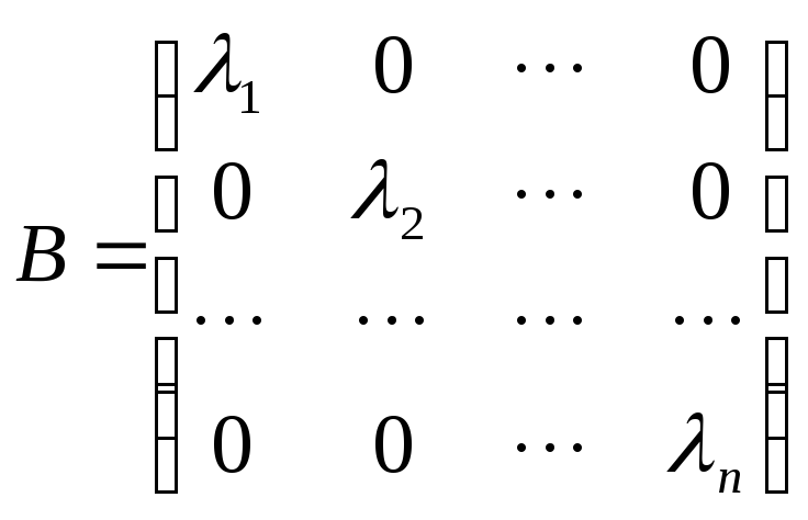
The canonical form of the quadratic form obviously means that the matrix A has a diagonal appearance:

Let's consider some linear transformation X = SY, where S is a square matrix of order n, and the matrices - columns X and Y are:

The matrix S is called the linear transformation matrix. Let us note in passing that any matrix of nth order with a given basis corresponds to a certain linear operator.

The linear transformation X = SY replaces the variables x 1, x 2, x 3 with new variables y 1, y 2, y 3. Then:

where B = S T A S

The task of reduction to canonical form comes down to finding a transition matrix S such that matrix B takes on a diagonal form:

So, quadratic form with matrix A after linear transformation of variables goes into quadratic form from new variables with matrix IN.

Let's turn to linear operators. Each matrix A for a given basis corresponds to a certain linear operator A . This operator obviously has a certain system of eigenvalues ​​and eigenvectors. Moreover, we note that in Euclidean space the system of eigenvectors will be orthogonal. We proved in the previous lecture that in the eigenvector basis the matrix of a linear operator has a diagonal form. Formula (*), as we remember, is the formula for transforming the matrix of a linear operator when changing the basis. Let us assume that the eigenvectors of the linear operator A with matrix A - these are the vectors y 1, y 2, ..., y n.

And this means that if the eigenvectors y 1, y 2, ..., y n are taken as a basis, then the matrix of the linear operator in this basis will be diagonal

or B = S -1 A S, where S is the transition matrix from the initial basis ( e) to basis ( y). Moreover, in an orthonormal basis, the matrix S will be orthogonal.

That. to reduce a quadratic form to a canonical form, it is necessary to find the eigenvalues ​​and eigenvectors of the linear operator A, which has in the original basis the matrix A, which generates the quadratic form, go to the basis of the eigenvectors and construct the quadratic form in the new coordinate system.

Let's look at specific examples. Let's consider second order lines.

or

By rotating the coordinate axes and subsequent parallel translation of the axes, this equation can be reduced to the form (variables and coefficients are redesignated x 1 = x, x 2 = y):

1)
if the line is central, 1  0,  2  0

2)
if the line is non-central, i.e. one of i = 0.

Let us recall the types of second-order lines. Center lines:

Off-center lines:

5) x 2 = a 2 two parallel lines;

6) x 2 = 0 two merging lines;

7) y 2 = 2px parabola.

Cases 1), 2), 7) are of interest to us.

Let's look at a specific example.

Bring the equation of the line to canonical form and construct it:

5x 2 + 4xy + 8y 2 - 32x - 56y + 80 = 0.

The matrix of quadratic form is
. Characteristic equation:

Its roots:

Let's find the eigenvectors:

When  1 = 4:
u 1 = -2u 2 ; u 1 = 2c, u 2 = -c or g 1 = c 1 (2 i – j).

When  2 = 9:
2u 1 = u 2 ; u 1 = c, u 2 = 2c or g 2 = c 2 ( i+2j).

We normalize these vectors:

Let's create a linear transformation matrix or a transition matrix to the basis g 1, g 2:

- orthogonal matrix!

The coordinate transformation formulas have the form:

or

Let's substitute lines into our equation and get:

Let's make a parallel translation of the coordinate axes. To do this, select complete squares of x 1 and y 1:

Let's denote
. Then the equation will take the form: 4x 2 2 + 9y 2 2 = 36 or

This is an ellipse with semi-axes 3 and 2. Let's determine the angle of rotation of the coordinate axes and their shift in order to build an ellipse in the old system.

P sharp:

Check: at x = 0: 8y 2 - 56y + 80 = 0 y 2 – 7y + 10 = 0. Hence y 1,2 = 5; 2

When y = 0: 5x 2 – 32x + 80 = 0 There are no roots here, i.e. there are no points of intersection with the axis X!

A quadratic form is called canonical if all i.e.

Any quadratic form can be reduced to canonical form using linear transformations. In practice, the following methods are usually used.

1. Orthogonal transformation of space:

Where - eigenvalues ​​of the matrix A.

2. Lagrange method - sequential selection of complete squares. For example, if

Then a similar procedure is performed with the quadratic form etc. If in quadratic form everything is but then after preliminary transformation the matter comes down to the procedure considered. So, if, for example, then we assume

3. Jacobi method (in the case when all major minors quadratic form are different from zero):

Any straight line on the plane can be specified by a first-order equation

Ax + Wu + C = 0,

Moreover, the constants A and B are not equal to zero at the same time. This first order equation is called general equation of a straight line. Depending on the values ​​of constants A, B and C, the following special cases are possible:

C = 0, A ≠0, B ≠ 0 – the straight line passes through the origin

A = 0, B ≠0, C ≠0 (By + C = 0) - straight line parallel to the Ox axis

B = 0, A ≠0, C ≠ 0 (Ax + C = 0) – straight line parallel to the Oy axis

B = C = 0, A ≠0 – the straight line coincides with the Oy axis

A = C = 0, B ≠0 – the straight line coincides with the Ox axis

The equation of a straight line can be presented in different forms depending on any given initial conditions.

A straight line in space can be specified:

1) as a line of intersection of two planes, i.e. system of equations:

A 1 x + B 1 y + C 1 z + D 1 = 0, A 2 x + B 2 y + C 2 z + D 2 = 0; (3.2)

2) by its two points M 1 (x 1, y 1, z 1) and M 2 (x 2, y 2, z 2), then the straight line passing through them is given by the equations:

= ; (3.3)

3) the point M 1 (x 1, y 1, z 1) belonging to it, and the vector a(m, n, p), collinear to it. Then the straight line is determined by the equations:

. (3.4)

Equations (3.4) are called canonical equations of the line.

Vector a called direction vector straight.

We obtain parametric equations of the line by equating each of the relations (3.4) to the parameter t:

x = x 1 +mt, y = y 1 + nt, z = z 1 + rt. (3.5)

Solving system (3.2) as a system of linear equations for unknowns x And y, we arrive at the equations of the line in projections or to given equations of the straight line:

x = mz + a, y = nz + b. (3.6)

From equations (3.6) we can go to the canonical equations, finding z from each equation and equating the resulting values:

.

From general equations (3.2) you can go to canonical ones in another way, if you find any point on this line and its direction vector n= [n 1 , n 2 ], where n 1 (A 1, B 1, C 1) and n 2 (A 2 , B 2 , C 2 ) - normal vectors of given planes. If one of the denominators m, n or R in equations (3.4) turns out to be equal to zero, then the numerator of the corresponding fraction must be set equal to zero, i.e. system

is equivalent to the system ; such a straight line is perpendicular to the Ox axis.

System is equivalent to the system x = x 1, y = y 1; the straight line is parallel to the Oz axis.

Every first degree equation with respect to coordinates x, y, z

Ax + By + Cz +D = 0 (3.1)

defines a plane, and vice versa: any plane can be represented by equation (3.1), which is called plane equation.

Vector n(A, B, C) orthogonal to the plane is called normal vector plane. In equation (3.1), the coefficients A, B, C are not equal to 0 at the same time.

Special cases of equation (3.1):

1. D = 0, Ax+By+Cz = 0 - the plane passes through the origin.

2. C = 0, Ax+By+D = 0 - the plane is parallel to the Oz axis.

3. C = D = 0, Ax + By = 0 - the plane passes through the Oz axis.

4. B = C = 0, Ax + D = 0 - the plane is parallel to the Oyz plane.

Equations of coordinate planes: x = 0, y = 0, z = 0.

A straight line may or may not belong to a plane. It belongs to a plane if at least two of its points lie on the plane.

If a line does not belong to the plane, it can be parallel to it or intersect it.

A line is parallel to a plane if it is parallel to another line lying in that plane.

A straight line can intersect a plane at different angles and, in particular, be perpendicular to it.

A point in relation to the plane can be located in the following way: belong to it or not belong to it. A point belongs to a plane if it is located on a straight line located in this plane.

In space, two lines can either intersect, be parallel, or be crossed.

The parallelism of line segments is preserved in projections.

If the lines intersect, then the points of intersection of their projections of the same name are on the same connection line.

Crossing lines do not belong to the same plane, i.e. do not intersect or parallel.

in the drawing, the projections of lines of the same name, taken separately, have the characteristics of intersecting or parallel lines.

Ellipse. An ellipse is a geometric locus of points for which the sum of the distances to two fixed points (foci) is the same constant value for all points of the ellipse (this constant value must be greater than the distance between the foci).

The simplest equation of an ellipse

Where a- semimajor axis of the ellipse, b- semiminor axis of the ellipse. If 2 c- distance between focuses, then between a, b And c(If a > b) there is a relationship

a 2 - b 2 = c 2 .

The eccentricity of an ellipse is the ratio of the distance between the foci of this ellipse to the length of its major axis

The ellipse has eccentricity e < 1 (так как c < a), and its foci lie on the major axis.

Equation of the hyperbola shown in the figure.

Options:
a, b – semi-axes;
- distance between focuses,
- eccentricity;
- asymptotes;
- headmistresses.
The rectangle shown in the center of the picture is the main rectangle; its diagonals are asymptotes.

This method consists of sequentially selecting complete squares in quadratic form.

Let the quadratic form be given

Recall that, due to the symmetry of the matrix

,

There are two possible cases:

1. At least one of the coefficients of squares is different from zero. Without loss of generality, we will assume (this can always be achieved by appropriate renumbering of variables);

2. All coefficients

but there is a coefficient different from zero (for definiteness, let it be).

In the first case transform the quadratic form as follows:

,

and all other terms are denoted by.

is a quadratic form of (n-1) variables.

They treat her in the same way and so on.

notice, that

Second case substitution of variables

comes down to the first.

Example 1: Reduce the quadratic form to canonical form through a non-degenerate linear transformation.

Solution. Let's collect all the terms containing the unknown , and add them to a complete square

.

(Because .)

or

(3)

or


(4)

and from unknown
form will take the form. Next we assume

or

and from unknown
form will take the canonical form

Let us resolve equalities (3) with respect to
:

or

Sequential execution of linear transformations
And
, Where

,

has a matrix

Linear transformation of unknowns
gives a quadratic form to the canonical form (4). Variables
associated with new variables
relations

We got acquainted with LU decomposition in workshop 2_1

Let's remember the statements from workshop 2_1

Statements(see L.5, p. 176)

This script is designed to understand the role of LU in the Lagrange method; you need to work with it in the EDITOR notepad using the F9 button.

And in the tasks attached below, it is better to create your own M-functions that help calculate and understand linear algebra problems (within the framework of this work)

Ax=X."*A*X % we get the quadratic form

Ax=simple(Ax) % simplify it

4*x1^2 - 4*x1*x2 + 4*x1*x3 + x2^2 - 3*x2*x3 + x3^2

% find the LU decomposition without rearranging the rows of the matrix A

% When converting a matrix to echelon form

%without row permutations, we get a matrix of M1 and U3

% U is obtained from A U3=M1*A,

% with this matrix of elementary transformations

0.5000 1.0000 0

0.5000 0 1.0000

%we get U3=M1*A, where

4.0000 -2.0000 2.0000

% from M1 it is easy to obtain L1 by changing the signs

% in the first column in all rows except the first.

0.5000 1.0000 0

0.5000 0 1.0000

% L1 is such that

A_=L1*U % this is the LU decomposition we need

% Elements on the main diagonal U -

% are coefficients of squares y i ^2

% in converted quadratic form

% in our case, there is only one coefficient

% means that in the new coordinates there will only be 4y 1 2 squared,

% for the remaining 0y 2 2 and 0y 3 2 coefficients are equal to zero

% columns of matrix L1 are the decomposition of Y by X

% in the first column we see y1=x1-0.5x2+0.5x3

% for the second we see y2=x2; according to the third y3=x3.

% if L1 is transposed,

% that is T=L1."

% T - transition matrix from (X) to (Y): Y=TX

0.5000 1.0000 0

1.0000 -0.5000 0.5000

% A2 – matrix of transformed quadratic form

% Note U=A2*L1." and A=L1* A2*L1."

4.0000 -2.0000 2.0000

1.0000 -0.5000 0.5000

% So, we got the decomposition A_=L1* A2*L1." or A_=T."* A2*T

% showing change of variables

% y1=x1-0.5x2+0.5x3

% and representation of quadratic form in new coordinates

A_=T."*A2*T % T=L1." transition matrix from (X) to (Y): Y=TX

isequal(A,A_) % must match the original A

4.0000 -2.0000 2.0000

2.0000 1.0000 -1.5000

2.0000 -1.5000 1.0000

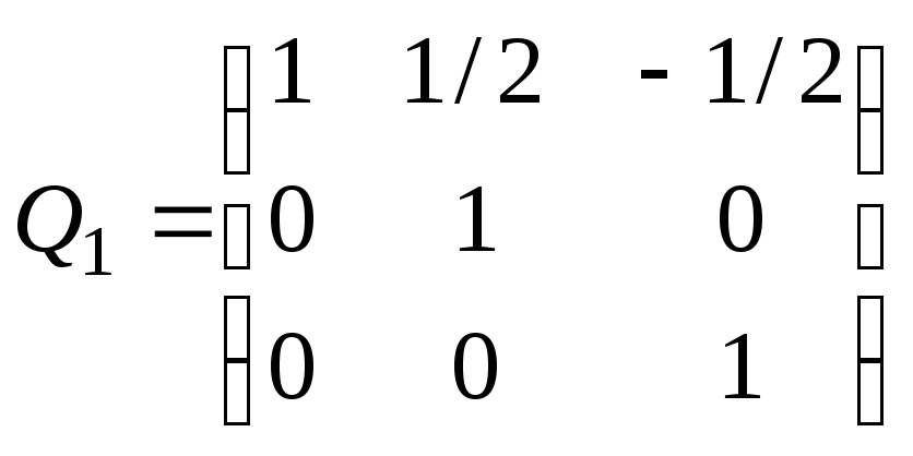
Q1=inv(T) % find the transition matrix from (Y) to (X)

% Let's find the transformation,

% quadratic Ax=X."*A*X

% to the new type Ay=(Q1Y)."*A*Q1Y=Y." (Q1."*A*Q1)*Y=Y." (U)*Y

Ay =4*y1^2 - y2*y3

x1 - x2/2 + x3/2

% second transformation matrix,

% which is much simpler to compile.

4*z1^2 - z2^2 + z3^2

% R=Q1*Q2, X=R*Z

R=Q1*Q2 % non-degenerate linear transformation

% bringing the operator matrix to canonical form.

det(R) % determinant is not equal to zero - the transformation is non-degenerate

4*z1^2 - z2^2 + z3^2 ok

4*z1^2 - z2^2 + z3^2

Let us formulate an algorithm for reducing quads ratical form to canonical form by orthogonal transformation:

Definition 10.4.Canonical view quadratic form (10.1) is called the following form: . (10.4)

Let us show that in a basis of eigenvectors, the quadratic form (10.1) takes on a canonical form. Let

- normalized eigenvectors corresponding to eigenvalues λ 1 ,λ 2 ,λ 3 matrices (10.3) in an orthonormal basis. Then the transition matrix from the old basis to the new one will be the matrix

. In the new basis the matrix A will take the diagonal form (9.7) (by the property of eigenvectors). Thus, transforming the coordinates using the formulas:

,

in the new basis we obtain the canonical form of a quadratic form with coefficients equal to the eigenvalues λ 1, λ 2, λ 3:

Remark 1. From a geometric point of view, the considered coordinate transformation is a rotation of the coordinate system, combining the old coordinate axes with the new ones.

Remark 2. If any eigenvalues ​​of the matrix (10.3) coincide, we can add a unit vector orthogonal to each of them to the corresponding orthonormal eigenvectors, and thus construct a basis in which the quadratic form takes the canonical form.

Let us bring the quadratic form to canonical form

x² + 5 y² + z² + 2 xy + 6xz + 2yz.

Its matrix has the form In the example discussed in Lecture 9, the eigenvalues ​​and orthonormal eigenvectors of this matrix are found:

Let's create a transition matrix to the basis from these vectors:

(the order of the vectors is changed so that they form a right-handed triple). Let's transform the coordinates using the formulas:

.

So, the quadratic form is reduced to canonical form with coefficients equal to the eigenvalues ​​of the matrix of the quadratic form.

Lecture 11.

Second order curves. Ellipse, hyperbola and parabola, their properties and canonical equations. Reducing a second order equation to canonical form.

Definition 11.1.Second order curves on a plane are called the lines of intersection of a circular cone with planes that do not pass through its vertex.

If such a plane intersects all the generatrices of one cavity of the cone, then in the section it turns out ellipse, at the intersection of the generatrices of both cavities – hyperbola, and if the cutting plane is parallel to any generator, then the section of the cone is parabola.

Comment. All second-order curves are specified by second-degree equations in two variables.

Ellipse.

Definition 11.2.Ellipse is the set of points in the plane for which the sum of the distances to two fixed points is F 1 and F tricks, is a constant value.

Comment. When the points coincide F 1 and F 2 the ellipse turns into a circle.

Let us derive the equation of the ellipse by choosing the Cartesian system

y M(x,y) coordinates so that the axis Oh coincided with a straight line F 1 F 2, beginning

r 1 r 2 coordinates – with the middle of the segment F 1 F 2. Let the length of this

segment is equal to 2 With, then in the chosen coordinate system

F 1 O F 2 x F 1 (-c, 0), F 2 (c, 0). Let the point M(x, y) lies on the ellipse, and

the sum of the distances from it to F 1 and F 2 equals 2 A.

Then r 1 + r 2 = 2a, But ,

therefore, introducing the notation b² = a²- c² and after carrying out simple algebraic transformations, we obtain canonical ellipse equation: (11.1)

Definition 11.3.Eccentricity of an ellipse is called the magnitude e=s/a (11.2)

Definition 11.4.Headmistress D i ellipse corresponding to the focus F i F i relative to the axis OU perpendicular to the axis Oh on distance a/e from the origin.

Comment. With a different choice of coordinate system, the ellipse can be specified not by the canonical equation (11.1), but by a second-degree equation of a different type.

Ellipse properties:

1) An ellipse has two mutually perpendicular axes of symmetry (the main axes of the ellipse) and a center of symmetry (the center of the ellipse). If an ellipse is given by a canonical equation, then its main axes are the coordinate axes, and its center is the origin. Since the lengths of the segments formed by the intersection of the ellipse with the main axes are equal to 2 A and 2 b (2a>2b), then the main axis passing through the foci is called the major axis of the ellipse, and the second main axis is called the minor axis.

2) The entire ellipse is contained within the rectangle

3) Ellipse eccentricity e< 1.

Really,

4) The directrixes of the ellipse are located outside the ellipse (since the distance from the center of the ellipse to the directrix is a/e, A e<1, следовательно, a/e>a, and the entire ellipse lies in a rectangle)

5) Distance ratio r i from ellipse point to focus F i to the distance d i from this point to the directrix corresponding to the focus is equal to the eccentricity of the ellipse.

Proof.

Distances from point M(x, y) up to the foci of the ellipse can be represented as follows:

Let's create the directrix equations:

(D 1), (D 2). Then From here r i / d i = e, which was what needed to be proven.

Hyperbola.

Definition 11.5.Hyperbole is the set of points in the plane for which the modulus of the difference in distances to two fixed points is F 1 and F 2 of this plane, called tricks, is a constant value.

Let us derive the canonical equation of a hyperbola by analogy with the derivation of the equation of an ellipse, using the same notation.

|r 1 - r 2 | = 2a, from where If we denote b² = c² - a², from here you can get

- canonical hyperbola equation. (11.3)

Definition 11.6.Eccentricity a hyperbola is called a quantity e = c/a.

Definition 11.7.Headmistress D i hyperbola corresponding to the focus F i, is called a straight line located in the same half-plane with F i relative to the axis OU perpendicular to the axis Oh on distance a/e from the origin.

Properties of a hyperbola:

1) A hyperbola has two axes of symmetry (the main axes of the hyperbola) and a center of symmetry (the center of the hyperbola). In this case, one of these axes intersects with the hyperbola at two points, called the vertices of the hyperbola. It is called the real axis of the hyperbola (axis Oh for the canonical choice of the coordinate system). The other axis has no common points with the hyperbola and is called its imaginary axis (in canonical coordinates - the axis OU). On both sides of it are the right and left branches of the hyperbola. The foci of a hyperbola are located on its real axis.

2) The branches of the hyperbola have two asymptotes, determined by the equations

3) Along with hyperbola (11.3), we can consider the so-called conjugate hyperbola, defined by the canonical equation

for which the real and imaginary axis are swapped while maintaining the same asymptotes.

4) Eccentricity of the hyperbola e> 1.

5) Distance ratio r i from hyperbola point to focus F i to the distance d i from this point to the directrix corresponding to the focus is equal to the eccentricity of the hyperbola.

The proof can be carried out in the same way as for the ellipse.

Parabola.

Definition 11.8.Parabola is the set of points on the plane for which the distance to some fixed point is F this plane is equal to the distance to some fixed straight line. Dot F called focus parabolas, and the straight line is its headmistress.

To derive the parabola equation, we choose the Cartesian

coordinate system so that its origin is the middle

D M(x,y) perpendicular FD, omitted from focus on the directive

r su, and the coordinate axes were located parallel and

perpendicular to the director. Let the length of the segment FD

D O F x is equal to R. Then from the equality r = d follows that

because the

Using algebraic transformations, this equation can be reduced to the form: y² = 2 px, (11.4)

called canonical parabola equation. Magnitude R called parameter parabolas.

Properties of a parabola:

1) A parabola has an axis of symmetry (parabola axis). The point where the parabola intersects the axis is called the vertex of the parabola. If a parabola is given by a canonical equation, then its axis is the axis Oh, and the vertex is the origin of coordinates.

2) The entire parabola is located in the right half-plane of the plane Ooh.

Comment. Using the properties of the directrixes of an ellipse and a hyperbola and the definition of a parabola, we can prove the following statement:

The set of points on the plane for which the relation e the distance to some fixed point to the distance to some straight line is a constant value, it is an ellipse (with e<1), гиперболу (при e>1) or parabola (with e=1).

Related information.