The history of "Derivative". Slide number 3. I. Historical background. David Gilbert. The general concept of derivative was made independently almost simultaneously. The end of the 16th - mid-17th centuries was marked by the enormous interest of scientists in explaining movement and finding the laws to which it obeys. Questions about determining and calculating the speed of movement and its acceleration have become more acute than ever. The solution to these questions led to the establishment of a connection between the problem of calculating the speed of a body and the problem of drawing a tangent to a curve describing the dependence of the distance traveled on time. English physicist and mathematician I. Newton. German philosopher and mathematician G. Leibniz.
Slide 10 from the presentation “Calculation of derivatives” for algebra lessons on the topic “Calculating the derivative”Dimensions: 960 x 720 pixels, format: jpg. To download a free slide for use in an algebra lesson, right-click on the image and click “Save Image As...”. You can download the entire presentation “Calculation of derivatives.ppt” in a 220 KB zip archive.
Download presentationDerivative calculation
“Derivative of a function at a point” - Programmed control. Theory issues. 0. Find the value of the derivative at point xo. 1) Find the angular coefficient of the tangent to the graph of the function f(x)=Cosх at point x=?/4. A. At the point. X.
“Prime function” - Repetition. Repeating and generalizing lesson (algebra 11th grade). Complete the task. Prove that the function F is an antiderivative of a function f on the set R. The main property of an antiderivative. Find the general form of the antiderivative for the function. Formulate: Definition of antiderivative. Rules for finding an antiderivative.
“Derivative of an exponential function” - www.thmemgallery.com. 11th grade. Rules of differentiation. Theorem 1. The function is differentiable at each point of the domain of definition, and. Derivative of an exponential function. Application of the derivative when studying a function. Theorem 2. Tangent equation. Derivatives of elementary functions. The natural logarithm is the logarithm to base e:
“Calculation of derivatives” - Oral warm-up, repetition of the rules for calculating derivatives (slide No. 1) 3. Practical part. Today's lesson will use presentations. 2. Activation of knowledge. The operation of finding the derivative is called differentiation. Slide No. 1. Student self-esteem. Main stages of the lesson Organizational moment.
“The geometric meaning of the derivative” - B. The geometric meaning of the increment of a function. S. So, the geometric meaning of the relation at. A. Slide 10. K – angular coefficient of the straight line (secant). Determination of the derivative of a function (To the textbook by A.N. Kolmogorov “Algebra and the beginnings of analysis 10-11”). The purpose of the presentation is to ensure maximum clarity of the topic.
The derivative of a function at a point is a basic concept in differential calculus. It characterizes the rate of change of the function at a specified point. The derivative is widely used in solving a number of problems in mathematics, physics, and other sciences, especially in studying the speed of various types of processes.
Basic definitions
The derivative is equal to the limit of the ratio of the increment of the function to the increment of the argument, provided that the latter tends to zero:
$y^(\prime)\left(x_(0)\right)=\lim _(\Delta x \rightarrow 0) \frac(\Delta y)(\Delta x)$
Definition
A function that has a finite derivative at some point is called differentiable at a given point. The process of calculating the derivative is called differentiation of function.
Historical background
The Russian term “derivative of a function” was first used by the Russian mathematician V.I. Viskovatov (1780 - 1812).
The designation of an increment (argument/function) with the Greek letter $\Delta$ (delta) was first used by the Swiss mathematician and mechanic Johann Bernoulli (1667 - 1748). The notation for the differential, derivative $d x$ belongs to the German mathematician G.W. Leibniz (1646 - 1716). The manner of denoting the time derivative with a dot over the letter - $\dot(x)$ - comes from the English mathematician, mechanic and physicist Isaac Newton (1642 - 1727). The short designation of a derivative by a prime - $f^(\prime)(x)$ - belongs to the French mathematician, astronomer and mechanic J.L. Lagrange (1736 - 1813), which he introduced in 1797. The partial derivative symbol $\frac(\partial)(\partial x)$ was actively used in his works by the German mathematician Karl G.Ya. Jacobi (1805 - 1051), and then the outstanding German mathematician Karl T.W. Weierstrass (1815 - 1897), although this designation had already been encountered earlier in one of the works of the French mathematician A.M. Legendre (1752 - 1833). The symbol of the differential operator $\nabla$ was invented by the outstanding Irish mathematician, mechanic and physicist W.R. Hamilton (1805 - 1865) in 1853, and the name "nabla" was proposed by the self-taught English scientist, engineer, mathematician and physicist Oliver Heaviside (1850 - 1925) in 1892.


Https://ppt4web.ru/images/1345/36341/310/img0.jpg" alt=" Presentation on the topic: Derivative. Completed by 11th grade students: Chelobitchikova Mar." title="Presentation on the topic: Derivative. Completed by 11th grade students: Chelobitchikova Mar.">!}
Slide description:
Slide no. 2

Slide description:
Slide no. 3

Slide description:
From history: In the history of mathematics, several stages in the development of mathematical knowledge are traditionally distinguished: Formation of the concept of a geometric figure and number as an idealization of real objects and sets of homogeneous objects. The advent of counting and measurement, which made it possible to compare different numbers, lengths, areas and volumes. Invention of arithmetic operations. Accumulation by empirical means (by trial and error) of knowledge about the properties of arithmetic operations, about methods of measuring areas and volumes of simple figures and bodies. The Sumerian-Babylonian, Chinese and Indian mathematicians of antiquity made great progress in this direction. The emergence of a deductive mathematical system in ancient Greece, which showed how to obtain new mathematical truths based on existing ones. The crowning achievement of ancient Greek mathematics was Euclid's Elements, which served as the standard of mathematical rigor for two millennia. Mathematicians from Islamic countries not only preserved ancient achievements, but were also able to synthesize them with the discoveries of Indian mathematicians, who advanced further than the Greeks in number theory. In the 16th-18th centuries, European mathematics was revived and went far ahead. Its conceptual basis during this period was the belief that mathematical models are a kind of ideal skeleton of the Universe, and therefore the discovery of mathematical truths is at the same time the discovery of new properties of the real world. The main success along this path was the development of mathematical models of dependence (function) and accelerated motion (analysis of infinitesimals). All natural sciences were rebuilt on the basis of newly discovered mathematical models, and this led to colossal progress. In the 19th and 20th centuries, it became clear that the relationship between mathematics and reality was far from being as simple as it previously seemed. There is no generally accepted answer to a kind of "fundamental question in the philosophy of mathematics": to find the reason for the "incomprehensible effectiveness of mathematics in the natural sciences." In this, and not only in this respect, mathematicians were divided into many debating schools. Several dangerous trends have emerged: excessively narrow specialization, isolation from practical problems, etc. At the same time, the power of mathematics and its prestige, supported by the effectiveness of its application, are higher than ever before
Slide no. 4

Slide description:
Slide no. 5

Slide description:
Differentiability The derivative f"(x0) of a function f at a point x0, being a limit, may not exist or exist and be finite or infinite. A function f is differentiable at a point x0 if and only if its derivative at this point exists and is finite: For a function f differentiable at x0 in a neighborhood of U(x0) has the following representation: f(x) = f(x0) + f"(x0)(x − x0) + o(x − x0)
Slide no. 6

Slide description:
Remarks Let's call Δx = x − x0 the increment of the function argument, and Δy = f(x0 + Δx) − f(x0) the increment of the function value at the point x0. Then Let the function have a finite derivative at each point. Then the derivative function is defined. A function that has a finite derivative at a point is continuous at it. The reverse is not always true. If the derivative function itself is continuous, then the function f is called continuously differentiable and is written:
Slide no. 7

Slide description:
Geometric and physical meaning of the derivative Geometric meaning of the derivative. On the graph of the function, the abscissa x0 is selected and the corresponding ordinate f(x0) is calculated. An arbitrary point x is selected in the vicinity of the point x0. A secant line is drawn through the corresponding points on the graph of function F (the first light gray line C5). The distance Δx = x - x0 tends to zero, as a result the secant turns into a tangent (gradually darkening lines C5 - C1). The tangent of the angle α of the slope of this tangent is the derivative at the point x0.
Slide no. 8

Slide description:
Derivatives of higher orders The concept of a derivative of an arbitrary order is defined recursively. We assume that If a function f is differentiable at x0, then the first-order derivative is determined by the relation Let now the nth-order derivative f(n) be defined in some neighborhood of the point x0 and differentiable. Then
Slide no. 9

Slide description:
Methods of writing derivatives Depending on the goals, scope and mathematical apparatus used, various methods of writing derivatives are used. Thus, the nth order derivative can be written in the notation: Lagrange f(n)(x0), while for small n primes and Roman numerals are often used: f(1)(x0) = f"(x0) = fI( x0),f(2)(x0) = f""(x0) = fII(x0),f(3)(x0) = f"""(x0) = fIII(x0),f(4)(x0 ) = fIV(x0), etc. This notation is convenient because of its brevity and is widely used; Leibniz, a convenient visual notation of the ratio of infinitesimals: Newton, which is often used in mechanics for the time derivative of the coordinate function (for the spatial derivative, the notation is more often used Lagrange). The order of the derivative is indicated by the number of points over the function, for example: - the first order derivative of x with respect to t at t = t0, or - the second derivative of f with respect to x at the point x0, etc. Euler, using a differential operator (strictly speaking, a differential expression, while the corresponding functional space has not been introduced), and therefore is convenient in questions related to functional analysis: Of course, we must not forget that they all serve to designate the same objects:
Slide no. 10

Slide description:
Examples: Let f(x) = x2. Then Let f(x) = | x | . Then if then f"(x0) = sgnx0, where sgn denotes the sign function. If x0 = 0, then f"(x0) does not exist
Slide no. 11

Slide description:
Rules of differentiation The operation of finding the derivative is called differentiation. When performing this operation, you often have to work with quotients, sums, products of functions, as well as “functions of functions,” that is, complex functions. Based on the definition of derivative, we can derive differentiation rules that make this work easier. (the derivative of a sum is equal to the sum of its derivatives) (from here, in particular, it follows that the derivative of the product of a function and a constant is equal to the product of the derivative of this function and a constant) If the function is given parametrically: then,
Derivative of a function Teacher of GAPOU RO "RKTM" Kolykhalina K.A. Increment of argument, increment of function Let x be an arbitrary point lying in some neighborhood of a fixed point x0. The difference x-x0 is called the increment of the independent variable (or increment of the argument) at the point x0 and is denoted ∆x. ∆х = x – x0 – increment of the independent variable. The increment of a function f at a point x0 is the difference between the values of the function at an arbitrary point and the value of the function at a fixed point. f(х) – f(х0)=f(х0+∆х) – f(х0) – increment of function f∆f=f(x0+∆x) – f(x0) Determination of the derivative Derivative of the function y= f(x) at the point x =x0 is the limit of the ratio of the increment of the function ∆y at this point to the increment of the argument ∆x, as the increment of the argument tends to zero. Algorithm for calculating the derivative The derivative of the function y= f(x) can be found according to the following scheme: 1. Give the argument x an increment ∆x≠0 and find the incremented value of the function y+∆y= f(x+∆x). 2. Find the increment of the function ∆y= f(x+∆x) - f(x). 3. We compose the relation 4. We find the limit of this relation at ∆x⇾0, i.e. (if this limit exists). Determination of the derivative of a function at a given point. Its geometric meaning
k – angular coefficient of the straight line (secant)
Tangent
Geometric meaning of derivative
The derivative of a function at a given point is equal to the slope of the tangent drawn to the graph of the function at this point.
Physical meaning of the derivative 1. The problem of determining the speed of movement of a material particle Let a point move along a certain straight line according to the law s= s(t), where s is the distance traveled, t is time, and it is necessary to find the speed of the point at the moment t0. By the moment of time t0, the distance traveled is equal to s0 = s(t0), and by the moment (t0 +∆t) – the path s0 + ∆s=s(t0 +∆t). Then over the interval ∆t the average speed will be. The smaller ∆t, the better the average speed characterizes the movement of the point at the moment t0. Therefore, under speed of the point at time t0 should be understood as the limit of the average speed for the period from t0 to t0 +∆t, when ∆t⇾0, i.e. 2. PROBLEM ABOUT THE RATE OF A CHEMICAL REACTION Let a substance undergo a chemical reaction. The amount of this substance Q changes during the reaction depending on time t and is a function of time. Let the amount of a substance change by ∆Q during time ∆t, then the ratio will express the average rate of a chemical reaction during time ∆t, and the limit of this ratio is the rate of the chemical reaction at a given time t.3. THE PROBLEM OF DETERMINING THE RADIOACTIVE DECAY RATE
If m is the mass of a radioactive substance and t is time, then the phenomenon of radioactive decay at time t, provided that the mass of the radioactive substance decreases over time, is characterized by the function m = m(t).
The average decay rate over time ∆t is expressed by the ratio
and the instantaneous decay rate at time t
Physical meaning of the derivative of a function at a given point
Derivatives of basic elementary functions Basic rules of differentiation Let u=u(x) And v=v(x) – differentiable functions at point x. 1) (u v) = u v 2) (uv) = uv +uv (cu) = cu 3) , If v 0
The history of the emergence of the concept of derivative
Functions, bounds, derivative, and integral are basic calculus concepts taught in high school courses. And the concept of derivative is inextricably linked with the concept of function.
The term “function” was first proposed by a German philosopher and mathematician to characterize different segments connecting the points of a certain curve in 1692. The first definition of a function, which was no longer associated with geometric concepts, was formulated in 1718. Pupil of Johann Bernoulli
in 1748. clarified the definition of function. Euler is credited with introducing the symbol f(x) to denote a function.A strict definition of the limit and continuity of a function was formulated in 1823 by the French mathematician Augustin Louis Cauchy . The definition of continuity of a function was formulated even earlier by Cauchy by the Czech mathematician Bernard Bolzano. According to these definitions, on the basis of the theory of real numbers, a rigorous justification of the basic principles of mathematical analysis was carried out.
The discovery of the approaches and foundations of differential calculus was preceded by the work of a French mathematician and lawyer, who in 1629 proposed methods for finding the largest and smallest values of functions, drawing tangents to arbitrary curves, and actually relying on the use of derivatives. This was also facilitated by the work that developed the coordinate method and the foundations of analytical geometry. Only in 1666 and somewhat later did they construct the theory of differential calculus independently of each other. Newton came to the concept of derivative by solving problems about instantaneous velocity, and , by considering the geometric problem of drawing a tangent to a curve. and investigated the problem of maxima and minima of functions.
Integral calculus and the very concept of an integral arose from the needs of calculating the areas of plane figures and volumes of arbitrary bodies. The ideas of integral calculus originate in the works of ancient mathematicians. However, this is evidenced by the “method of exhaustion” of Eudoxus, which he later used in the 3rd century. BC The essence of this method was to calculate the area of a flat figure and, by increasing the number of sides of the polygon, find the boundary into which the areas of the stepped figures were directed. However, for each figure, the calculation of the limit depended on the choice of a special technique. But the problem of a general method for calculating the areas and volumes of figures remained unsolved. Archimedes had not yet explicitly used the general concept of boundary and integral, although these concepts were used implicitly.
In the 17th century , who discovered the laws of planetary motion, the first attempt to develop ideas was successfully carried out. Kepler calculated the areas of flat figures and the volumes of bodies, based on the idea of decomposing a figure and a body into an infinite number of infinitesimal parts. These parts, as a result of addition, consisted of a figure whose area is known and allows one to calculate the area of the desired one. The so-called “Cavaglieri principle” entered the history of mathematics, with the help of which areas and volumes were calculated. This principle received theoretical justification later with the help of integral calculus.
The ideas of other scientists became the basis on which Newton and Leibniz discovered integral calculus. The development of integral calculus continued much later. Pafnutiy Lvovich Chebyshev
developed methods for integrating certain classes of irrational functions.
The modern definition of an integral as the limit of integral sums is due to Cauchy. Symbol